3.9 Linear or Affine Approximation

In single variable calculus, we learned that the tangent line to the graph of \(y=f(x)\) at \(x=x_0\) gives a good approximation of \(f(x)\) near \(x_0\) if \(f'(x_0)\) exists: \[f(x)\approx
L(x)=f(x_0)+f'(x_0)(x-x_0).\] Here \(L(x)\) is called the linearization [1] of \(f\) at the point \(x\) (see Fig. 1).

Figure 1 : Linearization in 2D-The tangent plane at \((x_0,y_0,f(x_0,y_0))\) is close to the graph of \(f\) for points \((x,y)\) close to \((x_0,y_0)\)

Similarly, for 2D problems, the tangent plane to the graph of \(z=f(x,y)\) at the point \(P=(x_0,y_0,z_0)\) gives a good approximation to the function near \((x_0,y_0)\) if the function is “smooth enough” (see Fig. 2):

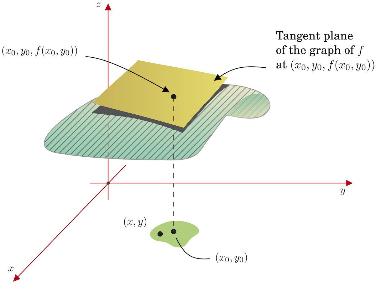
Figure 2: The tangent plane at \((x_0 , y_0 , f (x_0 , y_0 ))\) is close to the graph of \(f\) for points \((x, y)\) close to \((x_0 , y_0 )\)

Definition 1. If \(z=f(x,y)\), the function \(L(x,y)\) which is given by the following equation is called the linearization of \(f\) at \((x_0,y_0)\) \[L(x,y)=f(x_0,y_0)+f_x(x_0,y_0)(x-x_0)+f_y(x_0,y_0)(y-y_0).\] If \(f\) is “smooth enough”, then for \((x,y)\) near \((x_0,y_0):\) \[f(x,y)\approx L(x,y)\]

Example 1

Approximate the value of \(f(0.2,-0.1)\) given \(f(x,y)=\cos x\ e^{2y}\).

Solution

We can use the linear approximation of \(f\) at \((0,0)\), where \(f\) and its partial derivatives can be easily evaluated: \[f(0,0)=1\] \[\begin{aligned}
f_x(x,y)=-\sin x\ e^{2y}\Rightarrow &f_x(0,0)=0\\
f_y(x,y)=2\cos x\ e^{2y}\Rightarrow &f_y(0,0)=2\end{aligned}\] Therefore \(L(x,y)=1+0\times(x-0)+2\times(y-0)\), which approximates \(f(0.2,-0.1)\) \[f(0.2,-0.1)\approx
L(0,2,-0.1)=1+2\times(-0.1)=0.8\]

The exact value of \(f(0.2,-0.1)=0.8024\), which means the error in this approximation is \(\approx 0.3\%\)

Extension to Functions of More Than Two Variables

We can easily extend the concept of the linearization of functions of more than two variables. For example, if \(u=f(x,y,z)\), then its linearization at \((x_0,y_0,z_0)\) is given by:
\[{\small L(x,y,z)=f(x_0,y_0,z_0)+f_x(x_0,y_0,z_0)\cdot(x-x_0)+f_y(x_0,y_0,z_0)\cdot(y-y_0)+f_z(x_0,y_0,z_0)\cdot(z-z_0)}\]
or \[{\small L(x,y,z)=f(x_0,y_0,z_0)+\frac{\partial f}{\partial
x}(x_0,y_0,z_0)\cdot(x-x_0)+\frac{\partial f}{\partial y}(x_0,y_0,z_0)\cdot(y-y_0)+\frac{\partial f}{\partial
z}(x_0,y_0,z_0)\cdot(z-z_0)}\]

If \(u=f(x_1,\cdots,x_n)\), its linearization at the point \(\mathbf{p}=(a_1,\cdots, a_n)\) is \[L(x_1,\cdots,x_n)=
f(\mathbf{p})+\left.\frac{\partial f}{\partial x_1}\right|_{\mathbf{p}}(x-a_1)+\cdots+\left.\frac{\partial
f}{\partial x_n}\right|_{\mathbf{p}} (x-a_n)\]

In the following example, we want to know whether we can approximate a function with its linearization if it is not smooth enough?

Example 2

Given \[f(x,y)=\left\{\begin{array}{ll}
\dfrac{xy}{x^2+y^2} & \text{if } (x,y)\neq (0,0)\\
\\
0 & \text{if } (x,y)= (0,0)
\end{array}
\right.,\] using the linearization of \(f\) at \((0,0)\), approximate \(f(0.01,-0.01)\) and compare it with its exact value.

Graph of \(f(x,y)=\frac{xy}{x^2+y^2}\)

Solution

To calculate \(f_x(0,0)\) and \(f_y(0,0)\), we have to use the definition of partial derivatives: \[f_x(0,0)=\lim_{h\to
0}\frac{f(0+h,0)-f(0,0)}{h}=\lim_{h\to 0}\frac{\frac{h\times 0}{h^2+0^2}-0}{h}=\lim_{h\to
0}\frac{0-0}{h}=0,\] \[f_y(0,0)=\lim_{k\to
0}\frac{f(0,0+k)-f(0,0)}{k}=\lim_{k\to 0}\frac{\frac{ 0\times k}{0^2+k^2}-0}{h}=\lim_{k\to
0}\frac{0-0}{k}=0,\] Therefore the linearization of \(f\) at \((0,0)\) reads: \[L(x,y)=\underbrace{f(0,0)}_{=0}+\underbrace{f_x(0,0)}_{=0}
x+\underbrace{f_y(0,0)}_{=0} y=0,\] Therefore \(L(0.01,-0.01)=0\). However the exact value of \(f(0.01,-0.01)\) is \(-1/2\).

In this example, \(f(x,y)=0\) on the \(x\) and \(y\)-axes, \(f(x,y)=\frac{1}{2}\) on \(x=y\) and \(f(x,y)=-\frac{1}{2}\) on \(x=-y\).

This example shows even if \(f_x(x_0,y_0)\) and \(f_y(x_0,y_0)\) exist, the linearization does not need to be a good approximation for \(f\) near \((x_0,y_0)\).

[1] Here, we use “linearization” or “linear approximation” loosely. Note that \(L(x)\) is not a linear function unless \(f(x_0)=0\), because any linear function has to pass through the origin. More precisely we should say \(L(x)\) is an “affine function” and the approximation is the “affine approximation”. An affine function is a function composed of a linear function + a constant.