An important application of the derivatives is in solving various problems of optimization. We have learned how to determine the maximum or minimum values for functions of a single variable, and now in this section, we want to know how to determine the for functions of two or more variables. The problem of finding the extreme values for functions of several variables has similar features to that for functions of a single variable but it is often more complicated. So first let’s review what we already know about the of functions of one variable.
Review of Maxima and Minima of Single Variable Functions
Consider a function \(y=f(x)\):
- We say \(f\) has a if there exists \(x_0\) in its domain such that for all \(x\) in the domain of \(f\), \(f(x)\leq f(x_0)\) [respectively \(f(x)\geq f(x_0)\)]. \(f(x_0)\) is called the maximum value (the minimum value) of \(f\). The word “extremum” refer to either a maximum or a minimum.
- We say \(f\) has a at \(x_0\) if \(f(x)\leq f(x_0)\) [respectively \(f(x)\geq f(x_0)\)] for all \(x\) in the domain of \(f\) that are sufficiently close to \(x_0\).
- If \(f\) is continuous on a closed interval \([a,b]\), it takes on both its absolute maximum value and its absolute minimum value on that interval. If the interval is not closed or if \(f\) is not continuous on that interval, there is no guarantee that the function takes on its extreme values on that interval.
- If \(f(x_0)\) is a relative or absolute extreme value of \(f\), then the point \(x_0\) is one of three kinds of points:
- the point \(x_0\) is a stationary point; that is, \(f'(x_0)=0\),
- the point \(x_0\) is a rough point; that is, \(f'(x_0)\) does not exist, or
- the point \(x_0\) is one of the endpoints of the domain of \(f\).
- If \(f^{\prime\prime}(x)>0\) for every \(x\) in an interval \(I\), then the graph of \(f\) is concave up on \(I\).
- If \(f^{\prime\prime}(x)<0\) for every \(x\) in an interval \(I\), then the graph of \(f\) is concave down on \(I\).
- If \(f'(x_0)=0\) and \(f^{\prime\prime}(x_0)>0\), then \(f\) has a local minimum at \(x_0\).
- If \(f'(x_0)=0\) and \(f^{\prime\prime}(x_0)<0\), then \(f\) has a local maximum at \(x_0\).
- If \(f'(x_0)=0\) and \(f^{\prime\prime}(x_0)=0\), more information is required to conclude whether or not \(f\) has a local extremum at \(x_0\). In fact, the additional information is the behavior of higher order derivatives.The complete theorem is as follows. Suppose
\(f'(x_0)=\cdots =f^{(n-1)}(x_0)=0\) and \(f^{(n)}(x_0)\neq 0\).- If \(n\) is even and \(f^{(n)}(x_0)>0\), then \(f\) has a local minimum at \(x_0\).
- If \(n\) is even and \(f^{(n)}(x_0)<0\), then \(f\) has a local maximum at \(x_0\).
- If \(n\) is odd, then \(f\) does not have an extremum at \(x_0\).
Definitions of Maxima and Minima for Multivariable Functions
Now we are ready to talk about finding maxima and minima for functions of two or more variables.
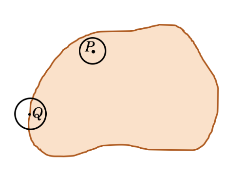
Consider a function \(z=f(x,y)\) defined on a set \(U\) in the \(xy\)-plane. We say \(f\) has a at the point \((x_0,y_0)\) of its domain \(U\) if \[f(x,y)\leq f(x_0,y_0)\] for all \((x,y)\) in \(U\). Absolute maximum corresponds to a highest point on the surface \(z=f(x,y)\). We say \(f\) has a relative maximum (or local maximum) at \((x_0,y_0)\) if \[f(x,y)\leq f(x_0,y_0)\] for all \((x,y)\) of \(U\) that are in a sufficiently small neighborhood of \((x_0,y_0)\). The value \(f(x_0,y_0)\) at a relative maximum does not have to be the greatest value of \(f(x,y)\) in the entire of \(U\) but the greatest value of \(f(x,y)\) if we restrict ourselves to points that are sufficiently close to \((x_0,y_0)\). The definitions of minimum (or more specifically absolute minimum) and relative minimum are analogous. Consider Fig. 1.

In a similar way we can define the maximum and minimum points for functions of three or more variables.
We say \(f\) has a maximum (or more specifically an absolute maximum) at the point \(\mathbf{x}_0\in U\) if \[f(\mathbf{x}_0)\geq f(\mathbf{x}),\] for all \(\mathbf{x}\in U\).
We say \(f\) has a relative maximum at the point \(\mathbf{x}_0\in U\), if there is a neighborhood \(V\) of \(\mathbf{x}_0\) such that for every
\(\mathbf{x}\in V\cap U\)
\[f(\mathbf{x}_0)\geq f(\mathbf{x}).\]
We say \(f\) has a minimum (or more specifically an absolute minimum) at the point \(\mathbf{x}_0\in U\) if \[f(\mathbf{x}_0)\geq f(\mathbf{x}),\] for all points \(\mathbf{x}\in U\).
We say \(f\) has a relative minimum (or local minimum) at the point \(\mathbf{x}_0\in U\) if there is a neighborhood \(V\) of \(\mathbf{x}_0\) such that for every \(\mathbf{x}\in V\cap U\)
\[f(\mathbf{x}_0)\leq f(\mathbf{x}),\]
A point which is either a (relative or absolute) maximum or minimum is called a (relative or absolute)
extremum.
- Every absolute maximum (respectively minimum) is also a relative maximum (minimum).
Bounded and Unbounded Sets
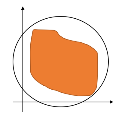
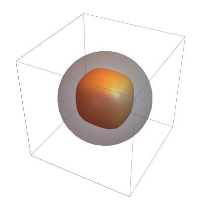
A set in \(\mathbb{R}\) is bounded if it is contained in an interval of finite length, and is unbounded otherwise. A set in \(\mathbb{R}^2\) is bounded if the entire set can be contained within a disk of finite radius, and is called unbounded if there is no disk that contains all the points of the set. Similarly, a set of \(\mathbb{R}^3\) is bounded if the entire set can be contained within a sphere of finite radius, and is unbounded otherwise. In general, A set in \(\mathbb{R}^n\) is bounded if the entire points of the set are contained inside a ball \(|\mathbf{x}|^2=x_1^2+x_2^2+\cdots+x_n^2\leq R^2\) of finite radius \(R\).
The Extreme Value Theorem
The following theorem assures us that a continuous function in a closed and bounded set takes on its extreme values.
In the conditional statement “if \(P\) then \(Q\)” or “\(P\) implies \(Q\)” (written as \(P \rightarrow Q\) ), we say \(P\) is a sufficient condition for \(Q\) and \(Q\) is necessary condition for \(P\). Also note that “if \(P\) then \(Q\)” is equivalent to “if \(Q\) is false, then \(P\) is false.”
Finding Extrema
Calculus gives us the necessary conditions for an interior point to be a relative extremum. Let \(f\) be a function of two variables \(x\) and \(y\) and let \((x_0,y_0)\) be an of the domain of \(f\). If \(f\) has a relative maximum or minimum at \((x_0,y_0)\) and if \(f_x(x_0,y_0)\) and \(f_y(x_0,y_0)\) exist, then
\[\overrightarrow{\nabla} f(x_0,y_0)=\mathbf{0} \quad \quad (\text{that is } f_x(x_0,y_0)=f_y(x_0,y_0)=0).\]
If we define a single-variable function \(F(x)=f(x,y_0)\) (see Fig. 3(a)), then \(F'(x)=f_x(x_0,y_0)\). If \((x_0,y_0)\) is a relative maximum point, then for all \((x,y)\) in the domain of \(f\) that are in a sufficiently small neighborhood of \((x_0,y_0)\), \(f(x_0,y_0)\geq f(x,y)\). Consequently, in that neighborhood \(F(x_0)\geq F(x)\). This means \(F\) has a relative maximum at \(x_0\). It follows from single variable calculus that \(F'(x_0)=0\); that is \(f_x(x_0,y_0)=0\) (Fig. 3(b)). The proof that \(f_y(x_0,y_0)=0\) is analogous.

At every relative extremum in the interior domain of a differentiable function \(f(x,y)\) we have
\[df=\underbrace{\frac{\partial f}{\partial x}}_{=0} dx+\underbrace{\frac{\partial f}{\partial y}}_{=0} dy=0,\]
for \((x,y)=(x_0,y_0)\) and all \(dx\) and \(dy\). Geometrically \(df=0\) means that the tangent plane at the point \((x_0,y_0,f(x_0,y_0))\) is horizontal (or perpendicular to the \(z\)-axis). See Fig.[fig:MaxMin-3]

We can easily generalize this result for functions of any number of independent variables. The proof of the following theorem is essentially the same as we discussed here, but is expressed in a different way.
Show the proof
Hide the proof
Suppose \(f\) has a relative maximum at \(\mathbf{x}_0\). We need to show \(f_{x_i}(\mathbf{x}_0)=0\). By the definition of a partial derivative
\[\frac{\partial f}{\partial x_i}(\mathbf{x}_0)=D_{\hat{\mathbf{e}}_i}f(\mathbf{x}_0)=\lim_{h\to 0}\frac{f(\mathbf{x}_0+t\hat{\mathbf{e}}_i)-f(\mathbf{x}_0)}{t},\]
where \(\hat{\mathbf{e}}_i\) as usual is the unit vector all of whose components are zero, except the \(i\)-th component, which is one.
Because \(f\) has a relative maximum at \(\mathbf{x}_0\), by Definition 1 we have \[f(\mathbf{x}_0+t\hat{\mathbf{e}}_i)- f(\mathbf{x}_0)\leq 0,\] whenever \(|t|\) is small enough, so that \(\mathbf{x}_0+t\hat{\mathbf{e}}_i\) is sufficiently close to \(\mathbf{x}_0\). If \(t\to 0^+\); that is, if \(t\) approaches 0 from the right, then \(t>0\); therefore:
\[\frac{f(\mathbf{x}_0+t\hat{\mathbf{e}}_i)-f(\mathbf{x}_0)}{t}\leq 0. \tag{*}\]
If \(t\to 0^-\); that is, \(t\) approaches 0 from the left, \(t<0\); therefore:
\[\frac{f(\mathbf{x}_0+t\hat{\mathbf{e}}_i)-f(\mathbf{x}_0)}{t}\geq 0. \tag{**}\]
If \(\frac{\partial f}{\partial x_i}(\mathbf{x}_0)\) exists, both inequalities (*) and (**) must hold. Therefore, we must have
\(\frac{\partial f}{\partial x_i}(\mathbf{x}_0)=0.\)
The proof when \(f\) has a relative minimum at \(\mathbf{x}_0\) is very similar. \(\blacksquare\)
It follows from Theorem 2 that if a function has a relative extremum at an interior point of its domain and if its partial derivatives at that point exist, the point must be a stationary point of the function. Theorem 2 does not talk about the points where the partial derivatives do not exist and the points on the boundary. That is, it is possible for a function to assume its (relative or absolute) extreme value at a point where at least one of the first partial derivatives does not exist (Fig. 5(a)) or at a boundary point (Fig. 5(b)).


(a) Maximum occurs at a rough point.
(b) Extrema occur at two boundary points.
Figure 5.
- A point at which at least one of the partial derivatives does not exist is called a rough point. In other words, at a rough point, the gradient does not exist.
- Stationary points and rough points constitute critical points.
- From the above discussion, we conclude that to determine the extreme values of a function, we should search them among stationary points, rough points, and boundary points.
A function \(f\) has a relative or absolute extremum at a point \(\mathbf{x}_0\) of its domain only if \(\mathbf{x}_0\) is one of the three types of points:
- \(\mathbf{x}_0\) is a stationary point of \(f\); that is, \(\overrightarrow{\nabla} f(\mathbf{x}_0)=\mathbf{0}\),
- \(\mathbf{x}_0\) is a rough point of \(f\); that is, \(\overrightarrow{\nabla} f(\mathbf{x}_0)\) does not exist, or
- \(\mathbf{x}_0\) is on the boundary of the domain of \(f\).
\[\overrightarrow{\nabla} f(x,y)=(2x, 2y).\]
The gradient exists everywhere; therefore, there is no rough point. Both components of the gradient are zero only at \((0,0)\); that is, \((0,0)\) is the only critical point of \(f\). Because \(f(0,0)=0\) and the value of \(f(x,y)\) is always greater than or equal to zero, \(f\) has an absolute minimum at the origin. The value of \(f\) increases unboundedly when we go away from the origin. So there is no absolute maximum.

and they become zero at the origin. The function has a maximum at the origin, because at all \((x,y)\neq (0,0)\) the quantity \(1-x^2-y^2\) under the square root is less than 1 which occurs at the origin.
The domain of \(f\) is \(1-x^2-y^2\geq 0\) or \(x^2+y^2\leq 1\), which is a disk of radius 1 and centered at the origin. On the boundary of the domain (i.e. \(x^2+y^2=1\)), \(f\) is zero. The absolute minimum value of \(f\) occurs on the boundary because the minimum of the square root is zero.

\[\frac{\partial f}{\partial x}=\frac{x}{\sqrt{x^2+y^2}},\quad \frac{\partial f}{\partial y}=\frac{y}{\sqrt{x^2+y^2}}.\]
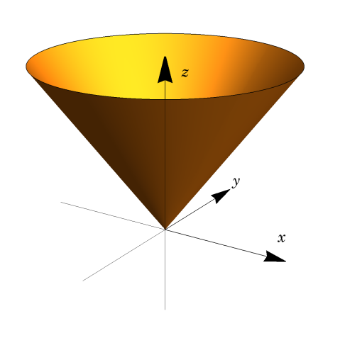
The partial derivatives are not both zero if \((x,y)\neq (0,0)\). Because \(\frac{\partial f}{\partial x}(0,0)\) and \(\frac{\partial f}{\partial y}(0,0)\) do not exist, \((0,0)\) is a rough point. The value of \(f\) at \((0,0)\) is zero. This is the minimum value the square root. Thus, \(f\) has an absolute minimum at the origin. The graph of \(f\) is a circular cone, \(f\) increases unboundedly when \(|(x,y)|\to\infty\) and does not have a maximum.
(a) We have
\[\begin{align} f(x,y)&=(x-a_1)^2+(y-b_1)^2+(x-a_2)^2+(y-b_2)^2+(x-a_3)^2+(y-b_3)^2\\ &=\sum_{i=1}^3 \left[(x-a_i)^2+(y-b_i)^2\right]\end{align}\]
\[\Rightarrow \frac{\partial f}{\partial x}=2(x-a_1+x-a_2+x-a_3),\quad \frac{\partial f}{\partial y}=2(y-b_1+y-b_2+y-b_3)\]
Solving \(\frac{\partial f}{\partial x}=0\) and \(\frac{\partial f}{\partial y}=0\) gives \(x=(a_1+a_2+a_3)/3\) and \(y=(b_1+b_2+b_3)/3\). Therefore, the best location to minimize sum of the square distances is the centroid of the triangle formed by the cities (Fig. 6).

(b) We have
\[\begin{align} g(x,y)&=r_1+r_2+r_3\\ &=\sum_{i=1}^3 \sqrt{(x-a_i)^2+(y-b_i)^2}.\end{align}\]
Differentiating \(g\) and equating to zero, we obtain
\[\begin{align} \frac{\partial g}{\partial x}&=\frac{x-a_1}{r_1}+\frac{x-a_2}{r_2}+\frac{a-x_3}{r_3}=0,\\ \frac{\partial g}{\partial y}&=\frac{y-b_1}{r_1}+\frac{y-b_2}{r_2}+\frac{y-b_3}{r_3}=0.\end{align}\]
These equations are complicated to solve. However, we note that
\[\overrightarrow{\nabla} g=\overrightarrow{\nabla} r_1+\overrightarrow{\nabla} r_2+\overrightarrow{\nabla} r_3,\]
where
\[\overrightarrow{\nabla} r_i=\left(\frac{x-a_i}{r_i},\frac{y-b_i}{r_i}\right) \ \ (\text{for } i=1,2,3)\]
Also we note that these gradient vectors \(\overrightarrow{\nabla} r_i\) are unit vectors, \(|\overrightarrow{\nabla} r_i|=1\). Therefore, the vector sum of three unit vectors at the relative minimum has to be \(\mathbf{0}\). The only way for this to happen is when the angles between them are 360\(^\circ\)/3=120\(^\circ\) (as (b) and (c) in the following figure). So the solution probably is when the roads from the cities to the center make 120\(^\circ\) angles. There are other possibilities. Each function \(r_i\) has a rough point; that is, \(g\) has three rough points. The graph of \(r_i\) is a circular cone (see Example [Eg:MinCone]), which has been shifted \(a_i\) units in the \(x\)-direction and \(b_i\) units in the \(y\)-direction. Therefore, \(r_i\) has a rough point at \((a_i,b_i)\). This means that if we build the distribution center in one of the cities, we might have minimized the cost.
If the triangle formed by the cities has an angle larger than 120\(^\circ\), then a point inside the triangle such that the angles between the roads from the delivery center to the cities make 120\(^\circ\) does not exist. In this case, the best point is the city with the wide angle (see (c) in the following figure). Otherwise, a point inside the triangle would be the solution.
 |
 |
 |
| (a) | (b) | (c) |

Saddle Points
Theorem 2 states necessary conditions (not sufficient ones). Not every critical point is a relative extremum. See the following example.
The answer is that the origin is neither a relative maximum nor a relative minimum. Because any neighborhood of \((0,0)\)— no matter how small it is— include points from each quarter; \(f(0,0)=0\) but \(f(x,y)>0\) for any point in the first (when \(x>0, y>0\)) and third (when \(x<0, y<0\)) quarters and \(f(x,y)<0\) for any point in the second (when \(x<0, y>0\)) and forth (when \(x>0, y<0\)) quarters. Such a point is called a saddle point.
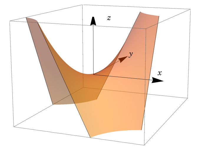
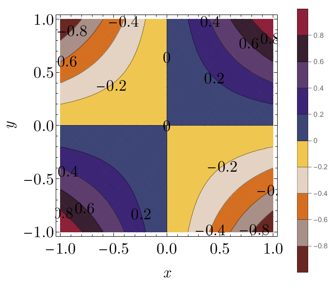
Figure 7.
Saddle points are somewhat analogous to the points of inflection for functions of one variable.
Second Partials Test
To figure out whether a critical point is a maximum, a minimum or a saddle point, we may graph the function but what if we do not have access to a graphing application or what can we do to classify the critical points of functions of three or more variables? Fortunately we can systematically use what is called the “second partials test.” This test is similar to the second derivative test for functions of one variable. Because application of the second partial tests for functions of three or more variables is rather laborious, here we restrict ourselves to functions of two variables.
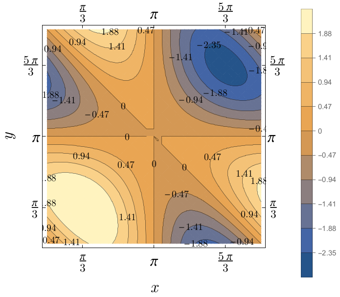
Let \((x,y)\) be a point (other than \((x_0,y_0)\)) in a neighborhood of \((x_0,y_0)\) where the second order partial derivatives of \(f\) are continuous. Using Taylor’s formula (Theorem 3), we can write Case I: \(\Delta=AC-B^2>0\). It follows from \(\Delta>0\) that \(A\neq 0\). Let’s define \(\phi(x,y)=f_{xx}(x,y)f_{yy}(x,y)-\left[f_{xy}(x,y)\right]^2\). We are given \(\Delta=\phi(x_0,y_0)>0\). Because \(f_{xx}, f_{yy}\), and \(f_{xy}\) are continuous in a neighborhood of \((x_0,y_0)\), say \(N_r(x_0,y_0)\), \(\phi(x,y)\) is also continuous in \(N_r(x_0,y_0)\). Hence, there is a neighborhood \(N_{r’}(x_0,y_0)\) of \((x_0,y_0)\) for some \(r’\leq r\) in which \(\phi(x,y)>0\) and \(f_{xx}(x,y)\) has the same sign as \(A\). Now consider only points \((x,y)=(x_0+h,y_0+k)\) that lie in \(N_{r’}(x_0,y_0)\). In this case \((x_0+h\theta,y_0+k\theta)\) for \(0<\theta<1\) also lies in \(N_{r’}(x_0,y_0)\); hence \(ac^2-b^2>0\) and \(a\) has the same sign as \(A\). The expression inside the square brackets in (*) is a quadratic form of \(h\) and \(k\). Because \(a\neq 0\), by completing the squares, we may rewrite (*) as \[\Delta f=\frac{1}{2a}\left[(ah+bk)^2+(ac-b^2)k^2\right]. \tag{**}\] The expression inside the square brackets in (**) is the sum of two squares. Therefore, \(\Delta f\) has the same sign as \(a\) (or \(A\)). Therefore, if \(A>0\), then \(\Delta f=f(x,y)-f(x_0,y_0)>0\); that is, \(f\) has a relative minimum at \((x_0,y_0)\). If \(A<0\), then \(\Delta f=f(x,y)-f(x_0,y_0)<0\); that is, \(f\) has a relative maximum at \((x_0,y_0)\). This proves parts (a) and (b) of the above theorem. Case II: \(\Delta=AC-B^2<0\). If \(A\neq 0\), we consider \((x,y)\) in a neighborhood of \((x_0,y_0)\) where \(\phi(x,y)<0\) and \(f_{xx}(x,y)\) has the same sign as \(A=f_{xx}(x_0,y_0)\). Again by completing the square, we can rewrite (*) as (**). Because \(ac-b^2<0\), the expression in square brackets in (**) is the difference of two squares. If we put \(k=0\) and \(h\neq 0\), \(\Delta f\) has the same sign as \(a\) (or, in turn, as \(A\)). Now if we put \(k\neq 0\) and \(h=-\frac{bk}{a}\), \(\Delta f\) has the sign opposite to that of \(A\). Therefore \(f\) has a saddle point at \((x_0,y_0)\). If \(A=0\) but \(C\neq 0\), again we can complete the square and rewrite (*) as \[\Delta f=\frac{1}{2c}\left[(ck+bh)^2-b^2h^2\right].\] Using the same argument as before (once putting \(h=0\) and \(k\neq 0\) and once \(h\neq 0\) and \(k=-bh/c\)), we can show that \(f\) has a saddle point at \((x_0,y_0)\). The last case we need to investigate is when \(\Delta<0\), and \(A=C=0\). If follows from \(\Delta<0\) that \(B\neq 0\). If we put \(h=k\), then Eq (*) becomes: \[\Delta f=\frac{h^2}{2}(a+2b+c).\] Taking the limit, we have: Case III: \(\Delta=AC-B^2=0\). Part (d) can be shown through examples. \(\blacksquare\) It follows from the first equation that \(y=x^2\). If we plug \(y=x^2\) into the second equation, we will arrive at \(3x^4-3x=3x(x^3-1)=0\), which gives us \(x=0\) or \(x=1\). Thus, there are two critical points \(O=(0,0)\) and \(P=(1,1)\). To determine if \(f\) has relative extrema at these points, we use the second partials test. The second order partial derivatives are \[f_{xx}(x,y)=6x, \quad f_{xy}(x,y)=-3,\quad f_{yy}(x,y)=6y.\] At \(O=(0,0)\): \[A=f_{xx}(0,0)=0,\quad B=f_{xy}(0,0)=-3,\quad f_{yy}(0,0)=0.\] Because At \(P=(1,1)\): \[A=f_{xx}(1,1)=6,\quad B=f_{xy}(1,1)=-3,\quad f_{yy}(1,1)=6.\] Because If we plug \(y=2k\pi+x\) (for \(k\in\mathbb{Z}\)) into the first equation, we obtain \[\cos x+\cos 2x=0 \tag{*}\] We know \(\cos 2x=2\cos^2 x-1\).1 If we plug this identity into (*), we obtain: \[2\cos^2 x+\cos x-1=0.\] This is a quadratic in \(\cos x\). Thus: The equation \(\cos x=\frac{1}{2}\) has two solutions in the interval \([0,2\pi)\): \(x=\frac{\pi}{3}\) or \(x=2\pi-\frac{\pi}{3}=\frac{5\pi}{3}\). Because \(y\) lies between 0 and \(2\pi\), we have to choose \(k=0\) and get \(y=x\); that is \(P_1=\left(\frac{\pi}{3},\frac{\pi}{3}\right)\) and \(P_2=\left(\frac{5\pi}{3},\frac{5\pi}{3}\right)\) are two critical points. The solution of \(\cos x=-1\) in the interval \([0,2\pi)\) is \(x=\pi\). Again because \(y\) lies between 0 and \(2\pi\), we have to choose \(k=0\) and find \(y=\pi\). The third critical point is \(P_3=\left(\pi,\pi\right)\) If we plug \(y=2k\pi-x\) into the first equation, we obtain \[\cos x+\underbrace{\cos(2k\pi)}_{=1}=0 \Rightarrow \cos x=-1,\] which is the same equation we had before. Hence the critical points are \(P_1=\left(\frac{\pi}{3},\frac{\pi}{3}\right), P_3=\left(\frac{5\pi}{3},\frac{5\pi}{3}\right)\) and \(P_2=\left(\pi,\pi\right)\). For each of these points, we use the second partials test. We have: At \(P_1=(\frac{\pi}{3},\frac{\pi}{3})\), we have: At \(P_2=(\frac{5\pi}{3},\frac{5\pi}{3})\), we have: At \(P_3=(\pi,\pi)\), we have: The graph of \(f\) is shown in Fig. 9. Figure 9. We mentioned that when \(\Delta=0\), the second partial test is inconclusive, and the function may have a maximum, minimum, or a saddle point at the critical point. In the previous example, \(f\) had a saddle point at a critical point where \(\Delta =0\). Now consider the following functions: \[g(x,y)=x^4+y^4,\quad \phi(x,y)=-(x^4+y^4),\quad \psi(x,y)=x^4-y^4.\] You can verify that the origin is a critical point of these functions; \(g\) has a relative minimum, \(\phi\) has a relative maximum, and \(\psi\) has a saddle point at the origin. See Fig. 10. 1 Alternatively, we can transform the sum into a product using \[\cos a+\cos b=2\cos\left(\frac{a+b}{2}\right) \cos\left(\frac{a-b}{2}\right).\] Thus \[\cos x+\cos 2x=2\cos\left(\frac{3x}{2}\right) \cos\left(\frac{x}{2}\right)=0.\] \[\cos \left(\frac{3x}{2}\right) =0 \Rightarrow \frac{3x}{2}=(2n+1)\frac{\pi}{2} \Rightarrow x=(2n+1)\frac{\pi}{3}\] \[\cos\left(\frac{x}{2}\right)=0 \Rightarrow \frac{x}{2}=(2n+1)\frac{\pi}{2} \Rightarrow x=(2n+1)\pi\] In the interval $[0,2\pi)$, we have $x=\frac{\pi}{3}$, or $x=\frac{5\pi}{3}$ or $x=\pi$. ↩
\[A=\frac{\partial^2 f}{\partial x^2}(x_0,y_0),\quad B=\frac{\partial^2 f}{\partial x \partial y}(x_0,y_0),\quad C=\frac{\partial^2 f}{\partial y^2}(x_0,y_0)\]
and let
\[\Delta =\det\, H(x_0,y_0)=\begin{bmatrix} A & B\\ B & C \end{bmatrix}=AC-B^2.\]
Then we have:
Show the proof
Hide the proof
\[\begin{align} \Delta f=&f(x_0+h,y_0+k)-f(x_0,y_0)\\ =&f_x(x_0,y_0) h+f_y(x_0,y_0) k+\frac{1}{2}\left[a h^2+2bhk +ck^2\right]\end{align}\]
where \(h=x-x_0\), \(k=y-y_0\), and \(a, b\) and \(c\) are the second order partial derivatives of \(f\) at some point \((x_0+h\theta,y_0+k\theta)\) for \(0<\theta<1\):
\[a=f_{xx}(x_0+h\theta,y_0+k\theta),\quad b=f_{xy}(x_0+h\theta,y_0+k\theta),\quad c=f_{yy}(x_0+h\theta,y_0+k\theta).\]
Because \((x_0,y_0)\) is a critical point, we have \(f_x(x_0,y_0)=f_y(x_0,y_0)=0\); thus,
\[\begin{align} \Delta f=\frac{1}{2}\left[a h^2+2bhk +ck^2\right] \tag{*}.\end{align}\]
\[\lim_{h\to 0}\frac{\Delta f}{h^2}=\lim_{h\to 0} \frac{a+2b+c}{2}=\frac{A+2B+C}{2}=B\neq 0.\]
Therefore \(\Delta f\) has the same sign as \(B\) for sufficiently small \(|h|\). If we put \(h=-k\), using the same argument, we can show that \(\Delta f\) has the same sign as \(-B\). This means we have shown \(f\) has a saddle point at \((x_0,y_0)\).
\[\begin{align} \left\{\begin{array}{l} f_x(x,y)=3x^2-3y=0\\ \\ f_y(x,y)=3y^2-3x=0 \end{array}\right.\end{align}\]
\[\Delta=\det\begin{bmatrix} 0 & -3\\ -3 & 0 \end{bmatrix} =AC-B^2=-9<0,\]
according to part (c) of Theorem 3, \(f\) has a saddle point at \(O=(0,0)\).
\[\Delta=\det\begin{bmatrix} 6 & -3\\ -3 & 6 \end{bmatrix} =AC-B^2=27>0,\]
and \(A=f_{xx}(1,1)=6>0\), according to part (a) of Theorem 3, \(f\) has a minimum at \(P=(1,1)\).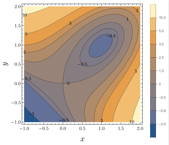
\[\begin{align} \left\{\begin{array}{l} f_x(x,y)=\cos x+\cos (x+y)=0\\ \\ f_y(x,y)=\cos y+\cos (x+y)=0 \end{array}\right.\end{align}\]
These equations together imply that \(\cos y=\cos x\); hence, \(y=2k\pi\pm x\).
\[\cos x=\frac{1}{4}(-1\pm\sqrt{1+8})=\frac{1}{2}\ \text{or}\ -1\]
\[\begin{align}f_{xx}(x,y)&=-\sin x-\sin (x+y), \\ \quad f_{xy}(x,y)&=-\sin(x+y), \\ \quad f_{yy}(x,y)&=-\sin y-\sin (x+y).\end{align}\]
\[\begin{align} A&=f_{xx}\left(\frac{\pi}{3},\frac{\pi}{3}\right)=-\sin\frac{\pi}{3}-\sin\frac{2\pi}{3}=-\sqrt{3}\\ B&=f_{xy}\left(\frac{\pi}{3},\frac{\pi}{3}\right)=-\sin \frac{2\pi}{3}=-\frac{\sqrt{3}}{2}\\ C&=f_{yy}\left(\frac{\pi}{3},\frac{\pi}{3}\right)=-\sin\frac{\pi}{3}-\sin\frac{2\pi}{3}=-\sqrt{3}.\end{align}\]
Thus
\[\Delta=\det\begin{bmatrix} -\sqrt{3} & -\frac{\sqrt{3}}{2}\\ \\ -\frac{\sqrt{3}}{2} & -\sqrt{3} \end{bmatrix}=3-\frac{3}{4}=\frac{9}{4}>0.\]
Because \(\Delta>0\) and \(A=-\sqrt{3}<0\), we can conclude that \(f\) has a maximum at \(P_1=\left(\frac{\pi}{3},\frac{\pi}{3}\right)\).
\[\begin{align} A&=f_{xx}\left(\frac{5\pi}{3},\frac{5\pi}{3}\right)=-\sin\frac{5\pi}{3}-\sin\frac{10\pi}{3}=\sqrt{3}\\ B&=f_{xy}\left(\frac{5\pi}{3},\frac{5\pi}{3}\right)=-\sin \frac{10\pi}{3}=\frac{\sqrt{3}}{2}\\ C&=f_{yy}\left(\frac{5\pi}{3},\frac{5\pi}{3}\right)=-\sin\frac{5\pi}{3}-\sin\frac{10\pi}{3}=\sqrt{3}.\end{align}\]
Thus
\[\Delta=\det\begin{bmatrix} \sqrt{3} & \frac{\sqrt{3}}{2}\\ \\ \frac{\sqrt{3}}{2} & \sqrt{3} \end{bmatrix}=3-\frac{3}{4}=\frac{9}{4}>0.\]
Because \(\Delta>0\) and \(A=\sqrt{3}>0\), we can conclude that \(f\) has a minimum at \(P_2=\left(\frac{5\pi}{3},\frac{5\pi}{3}\right)\).
\[\begin{align} A&=f_{xx}\left(\pi,\pi\right)=-\sin\pi-\sin2\pi=0\\ B&=f_{xy}\left(\pi,\pi\right)=-\sin 2\pi=0\\ C&=f_{yy}\left(\pi,\pi\right)=-\sin\pi-\sin{2\pi}=0.\end{align}\]
Thus
\[\Delta=\det\begin{bmatrix} 0 & 0\\ 0& 0 \end{bmatrix}=0.\] Because \(\Delta=0\), the second partial test is inconclusive. In this example, to investigate whether or not \(f\) has an extremum at \(P_3\), we can calculate the variation (increment) of \(f\) near \(P_3\):
\[\begin{align} \Delta f=f(\pi+h,\pi+k)-f(\pi,\pi)=\sin(\pi+h)+\sin(\pi+k)+\sin(2\pi+h+k)-\underbrace{f(\pi,\pi)}_{=0}\end{align}\]
Now we can use Taylor’s expansion
\[\begin{align} \Delta f=&-\sin h-\sin k+\sin(h+k)\\ =&-\left[h-\frac{h^3}{3}+\cdots\right]-\left[k-\frac{k^3}{3!}+\cdots\right]+\left[(h+k)-\frac{(h+k)^3}{3}+\cdots\right]\end{align}\]
To approximate \(\Delta f\), because \(h\) and \(k\) can be made as small as we desire, we just keep the dominant terms which are the terms with the lowest degree (i.e. the terms with the smallest power) and ignore the other terms as being negligible by comparison:
\[\begin{align} \Delta f \approx&\frac{h^3}{6}+\frac{k^3}{6}-\frac{(h+k)^3}{6}=-\frac{hk}{2}(h+k).\end{align}\]
If \(hk<0\) and \((h+k)>0\) (for example \(h=0.002\) and \(k=-0.001\)), \(\Delta f>0\) and if \(hk<0\) but \((h+k)<0\) (for example, \(h=-0.002\) and \(k=0.001\)), \(\Delta f<0\). Therefore, \(f\) has a saddle point at \(P_3=(\pi,\pi)\).