
- In many practical problems, we need to find the greatest (maximum) value or the least (minimum) value—there can be more than one of each—of a function.
- The maximum and minimum values of a function are called the extreme values or extrema of the function.
- Extremum is the singular form of extrema. The plural forms of maximum and minimum are maxima and minima, respectively.
- Differentiation can help us locate the extreme values of a function.
In calculus, there are two types of “maximum” and “minimum,” which are distinguished by the two prefixes: absolute and relative.
Absolute Maxima and Minima
The concepts of absolute maximum and minimum were introduced in Chapter 4. Let’s review the definitions.
Let the function \(f\) be defined on a set \(E\). We say \(f\) has an absolute maximum on \(E\) at a point \(p\) if \[f(x)\leq f(p)\quad\text{for all }x\text{ in }E,\] and an absolute minimum value on \(E\) at \(q\) if
\[f(x)\geq f(q)\quad\text{for all }x\text{ in }E.\]
Absolute maxima and absolute minima (plural forms of maximum and minimum) are also referred to as global maxima and global minima.
Previously, we learned that:
Theorem 1. The Extreme Value Theorem: If \(f\) is continuous on a closed interval \([a,b]\), then \(f\) attains both its absolute maximum \(M\) and absolute minimum \(m\) in \([a,b]\). That is, there are numbers \(p\) and \(q\) in \([a,b]\) such that \(f(p)=M\) and \(f(q)=m\).
We should emphasize that:
- The continuity of the function on an open interval (instead of a closed interval) is not sufficient to guarantee the existence of the absolute maximum and minimum of the function.
- If the function fails to be continuous even at one point in the interval \([a,b]\), the extreme value theorem may fail to be true (although a discontinuous function may have max and min).
For more information, see the Section on the Extreme Value Theorem.
Local (or Relative) Maxima and Minima


- Geometrically speaking local maxima and local minima are respectively the “peaks” and “valleys” of the curve.

Definition 1. A function \(f\) is said to have a local (or relative) maximum at a point \(c\) within its domain \(D\) if there is some open interval \(I\) containing \(c\) such that \[f(x)\leq f(c)\quad\text{for all }x\in{I}.\] The concept of local (or relative) minimum is similarly defined by reversing the inequality.
- Every absolute maximum or minimum that is not an endpoint of an interval is a local maximum or local minimum, respectively. An endpoint is precluded from being a local extremum because we cannot find an open interval around an endpoint that is contained in the domain of the function.

Because \(x_{2}\not\in Dom(f)\) , the function cannot have a maximum there. Moreover, it is evident that \(f(x_{4})\) is a local maximum. We claim that \(f(x_{6})\) is a local maximum because if we zoom in, we realize that for all \(x\) close enough to \(x_{6}\),
\[f(x)\leq f(x_{6}).\]

All the absolute and local extrema are shown in Figure 6.


- Notice that differentiability, or even continuity, of \(f\) at other points is not required.
- The geometrical interpretation of the above theorem is: At a local max or min, \(f\) either has no tangent, or $f$ has a horizontal tangent.
Show the proof
Hide the proof
We shall give the proof for the case of a local minimum at \(x=c\). According to the definition, we have \[f(c)\leq f(c+h)\] or \[0\leq f(c+h)-f(c)\] for all \(h\) sufficiently close to zero (that is, when \(c+h\) is near \(c\)). If \(f'(c)\) does not exist, there is nothing else to prove. So suppose \[f'(c)=\lim_{h\to0}\frac{f(c+h)-f(c)}{h}\] exists as a definite number. We need to show \(f'(c)=0\). When \(h\) is small, we have \[\frac{f(c+h)-f(c)}{h}\geq0\quad\text{if }h>0\] and \[\frac{f(c+h)-f(c)}{h}\leq0\quad\text{if }h<0\] because the numerator in both cases is either positive or zero (\(f(c+h)-f(c)\geq0\)). If we let \(h\to0^{+}\), from the first case, we have
\[f'(c)\geq0,\] and if we let \(h\to0^{-}\), from the second case, we have \[f'(c)\leq0.\] Because we have assumed that \(f'(c)\) exists, we must have the same limit in both cases, so \[0\leq f'(c)\leq0.\] This can happen only when \(f'(c)=0\). The proof for the case of a local maximum is similar.
The above theorem states a necessary condition for a local extremum. That the condition is not sufficient is evident from a glance at the point \((r,f(r))\) in Figure 9. The graph of \(f\) has a horizontal tangent at this point, but \(f\) does not have an extreme value at \(x=r\). As another example, consider: \(f(x)=x^{3}\)
\[f(x)=x^{3}\Rightarrow f'(x)=3x^{2}\]
\[f'(0)=0\] but \(x=0\) does not give either a local maximum or a local minimum of \(f\), as is obvious from the graph of \(y=x^{3}\) (Figure 10(a)). If \(g(x)=\sqrt[3]{x}\), then
\[g(x)=x^{1/3}\Rightarrow g'(x)=\frac{1}{3}x^{1/3-1}=\frac{1}{3}x^{-2/3}=\frac{1}{3\sqrt[3]{x^{2}}}\]
and \(g'(0)\) is not defined (we may say \(g'(0)=+\infty\)), but \(g(0)=0\) is not a local extremum (Figure 10(b)).

Critical Points
A number in the domain of the function at which the derivative is zero or the derivative does not exist has a special name. It is called a critical number.
Definition 2. Critical point: A point \(c\) in the domain of a function \(f\) is called a critical point (or critical number) of \(f\) if \[f'(c)=0\quad\text{or}\quad f'(c)\text{ does not exist.}\]
The number \(f(c)\) is called a critical value of \(f\).
- Recall that if \(f'(c)=+\infty\) or \(f'(c)=-\infty\), we say \(f'(c)\) does not exist because \(+\infty\) and \(-\infty\) are not numbers.
By the above definition, we can reword Fermat’s theorem as:
Fermat’s Theorem: If \(f(c)\) is a local maximum or a local minimum, then \(x=c\) is a critical number of \(f\).
- According to the above theorem, every single local extreme value is a critical value, but not every critical value is necessarily a local extreme value.

- We mentioned that every absolute extreme value, with the exception of an absolute extreme value that occurs at an endpoint, is also a local extreme value. Hence:
An absolute maximum or minimum of a function occurs either at a critical point or at an endpoint of its domain.

This provides us a method to find the absolute maximum and the absolute minimum of a differentiable function on a finite closed interval \([a,b]\).
Strategy for finding the absolute extrema of a continuous function \(f\) on a finite closed interval \([a,b]\):
- Step 1: Find \(f'(x)\)
- Step 2: Find all critical values: Set \(f'(x)=0\) and solve it for \(x\). Also find every value of \(x\) for which \(f'(x)\) does not exist. Evaluate \(f\) at each of these numbers that lie between \(a\) and \(b\).
- Step 3: Evaluate \(f(a)\) and \(f(b)\).
- Step 4: The largest value of \(f\) from Steps 2 and 3 is the absolute maximum of \(f\) and the least value of \(f\) from these steps is the absolute minimum of \(f\) on \([a,b]\).
\[f(2)=\frac{1}{3}(2^{3})-4(2)=-\frac{16}{3}\approx-5.333\] \[f(-2)=\frac{1}{3}(-2)^{3}-4(-2)=\frac{16}{3}\approx5.333\] Step 3:
Evaluating \(f\) at the endpoints
\[f(-3)=\frac{1}{3}(-3)^{3}-4(-3)=3\]
\[f(4)=\frac{1}{3}(4^{3})-4(4)=\frac{16}{3}\approx5.33\] Step 4: Comparing the critical values and the endpoint values.
| \(-3\) | \(-2\) | \(2\) | \(4\) | |
|---|---|---|---|---|
| \(f(x)\) | \(3\) | \(\frac{16}{3}\) | \(-\frac{16}{3}\) | \(\frac{16}{3}\) |
| max | min | max |
The absolute maximum of \(f\) on \([-3,4]\) is \(16/3\), which occurs at \(x=-2\) and \(x=4\), and its absolute minimum on this interval is \(-16/3\), which occurs at \(x=-2\). The graph of \(f\) is shown in Figure 11.

\[f(x)=x-3(x-1)^{2/3}\Rightarrow f'(x)=1-3\cdot\frac{2}{3}(x-1)^{-1/3}\] so \[f'(x)=1-\frac{2}{\sqrt[3]{x-1}}.\] Step 2: Finding the critical values of \(f\) \[f'(x)=0\]
\[1-\frac{2}{\sqrt[3]{x-1}}=0\]
\[\frac{1}{\sqrt[3]{x-1}}=\frac{1}{2}\]
\[\sqrt[3]{x-1}=2\] \[x-1=2^{3}=8\] \[x=9\] But \(x=9\) does not lie between \(-1\) and \(2\).
We notice that \(f'(x)\) does not exists when \(x=1\). Therefore, \(x=1\) is another critical point of \(f\), and \[f(1)=1-3(1-1)^{2/3}=1.\] Step 3: Evaluating \(f\) at the endpoints of the given interval
\[\begin{align} f(-1) & =-1-3(-2)^{2/3}\\ & =-1-3\sqrt[3]{4}\approx-5.76\end{align}\]
\[\begin{align} f(2) & =2-3(2-1)^{2/3}\\ & =2-3\\ & =-1\end{align}\]
Step 4: Comparing the critical values and the endpoint values.
| \(-1\) | \(1\) | \(2\) | |
|---|---|---|---|
| \(f(x)\) | \(-1-3\sqrt[3]{4}\) | \(1\) | \(-1\) |
| min | max |
Thus the absolute max of \(f\) on \([-1,2]\) is \(1\) , which occurs at \(x=1\) and the absolute min of \(f\) on that interval is \(1-3\sqrt[3]{4}\), which occurs at \(x=-1\). The graph of \(f\) is shown in Figure 12.

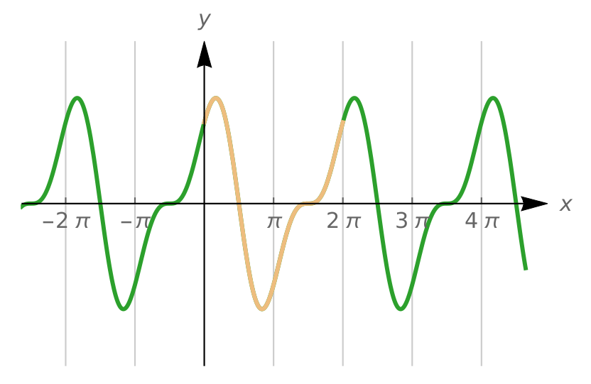
Step 1: \[f(x)=\sin2x+2\cos x\Rightarrow f'(x)=2\cos2x-2\sin x\] Step 2: \[f'(x)=2\cos2x-2\sin x=0\] We can express \(\cos2x\) in terms of \(\sin x\): \(\cos2x=1-2\sin^{2}x\) (see the section on Trigonometric Identities). Thus \[f'(x)=2(1-\sin^{2}x)-2\sin x=0\] \[-4\sin^{2}x-2\sin x+2=0\] This is a quadratic equation in terms of \(\sin x\). Let \(u=\sin x\). Thus
\[-4u^{2}-2u+2=0\]
\[\Rightarrow u=\frac{2\pm\sqrt{2^{2}-4(-4)2}}{2(-4)}=\frac{2\pm\sqrt{36}}{-8}\]
\[u=\frac{1}{2},\quad u=-1\] We have to solve \[\sin x=\frac{1}{2},\quad\sin x=-1\] when \(0\leq x\leq2\pi\).
\[\sin x=-\frac{1}{2}\Rightarrow x=\frac{\pi}{6},\quad x=\pi-\frac{\pi}{6}=\frac{5\pi}{6}\]
and \[\sin x=-1\Rightarrow x=\frac{3\pi}{2}.\] (See Figure 14(a,b))

Thus the critical points (or critical numbers) are
\[x=\frac{\pi}{6},\quad x=\frac{5\pi}{6},\quad x=\frac{3\pi}{2}.\] Let’s evaluate \(f\) at these points.
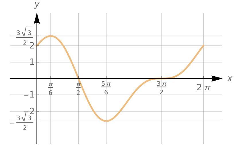
\[\begin{align} f\left(\frac{\pi}{6}\right) & =\sin\frac{\pi}{3}+2\cos\frac{\pi}{6}\\ & =\frac{\sqrt{3}}{2}+2\left(\frac{\sqrt{3}}{2}\right)\\ & =\frac{3\sqrt{3}}{2}.\end{align}\]
\[\begin{align} f\left(\frac{5\pi}{6}\right) & =\sin\frac{5\pi}{3}+2\cos\frac{5\pi}{6}\\ & =\sin\left(2\pi-\frac{\pi}{3}\right)+2\cos\left(\pi-\frac{\pi}{6}\right)\\ & =\sin\left(-\frac{\pi}{3}\right)-2\cos\frac{\pi}{6}\\ & =-\sin\frac{\pi}{3}-2\cos\frac{\pi}{6}\\ & =-\frac{\sqrt{3}}{3}-2\frac{\sqrt{3}}{2}\\ & =-\frac{3\sqrt{3}}{2}.\end{align}\]
Here we have used the identities \(\sin(2\pi+\theta)=\sin\theta\) and \(\cos(\pi-\theta)=-\cos\theta\) (see Trigonometric Identities).
\[\begin{align} f\left(\frac{3\pi}{2}\right) & =\sin3\pi+2\cos\frac{3\pi}{2}\\ & =0+0\\ & =0.\end{align}\]
Step 3: Evaluation of \(f\) at the endpoints
\[f(0)=\sin(2\cdot0)+2\cos0=0+2(1)=2\]
\[f(2\pi)=\sin(4\pi)+2\cos(2\pi)=0+2(1)=2.\] Step 4:
| \(f(x)\) | \(2\) | \(\frac{3\sqrt{3}}{2}\approx2.598\) | \(-\frac{3\sqrt{3}}{2}\approx-2.598\) | \(0\) | \(2\) |
| max | min |
The above table shows that the maximum value of \(f\) is \(3\sqrt{3}/2\) and its absolute minimum is \(-3\sqrt{3}/2\), which occur at \(x=\pi/6\) and \(x=5\pi/6\), respectively.
1\(x≤y\) means \(x<y\) or \(x=y.\), so we can write, for example, \(2≤2.\) Here \(f(x)=f(x_0)\) for all \(x\) in \(I\), and therefore we can write \(f(x)≤f(x_0)\) or \(f(x)≥f(x_0).\) ↗