3.3 Level Curves and Level Surfaces

Topographic (also called contour) maps are an effective way to show the elevation in 2-D maps. These maps are marked with contour lines or curves connecting points of equal height.

Figure 1: Topographic map of Stowe, Vermont, in the US. The brown contour lines represent the elevation. The contour interval is 20 feet.

The same idea can be used to represent a function $z = f (x, y)$ graphically. If the graph of the function $z = f (x, y)$ is cut by the horizontal (or level) plane $z = c$ , and if we project this intersection onto the $x y$ -plane, then we get a curve that consists of points $(x, y)$ for which $f (x, y) = c$ (Figure 2). Such a curve is called the level curve of height $c$ or the level curve with value $c$ and is denoted by $L (c)$ or by $f^{- 1} (c)$ . By drawing a number of level curves, we get what is called a contour plot or contour map, which provides a good representation of the function $z = f (x, y)$ .

Figure 2: The circle on the

x y

plane is the set of points for which

f (x, y) = c

In the next few examples, we will practice how to determine the contour curves. Let’s start with simple examples.

Recall that $(x - x_{0})^{2} + (y - y_{0})^{2} = R^{2}$ is the equation of a circle of radius $R$ centered at $(x_{0}, y_{0})$

Example 1

Sketch some level curves of $f (x, y) = x^{2} + y^{2}$ .

Solution

The level curves are graphs of equations of the form $f (x, y) = c$ ; that is,
$x^{2} + y^{2} = c .$ Because $x^{2}, y^{2} \geq 0$ , the above equation has a solution when $c \geq 0$ . When $c \geq 0$ , the above equation is the equation of a circle of radius $\sqrt{c}$ centered at $(0, 0)$ . When $c = 0$ , this equation gives the origin or a circle of radius 0. Figure 3 shows the graph and a number of the level curves of this function.

Figure 3(a): The graph of the function

z = f (x, y) = x^{2} + y^{2}

and the level curves

Figure 3(b): The level curves of

f

with different values of

c

Recall that $\frac{(x - x_{0})^{2}}{a^{2}} + \frac{(y - y_{0})^{2}}{b^{2}} = 1$ is the equation of an ellipse centered at $(x_{0}, y_{0})$ with semi major axis $a$ and semi minor axis $b$ (if $a \geq b$ ).

Example 2

Sketch some level curves of $f (x, y) = \frac{1}{4} (x - 1)^{2} + (y + 2)^{2}$ .

Solution

The level curve with value $c$ is obtained by setting $f (x, y) = c$ ; that is,
$\frac{1}{4} (x - 1)^{2} + (y + 2)^{2} = c .$ Obviously there is no level curve with value $c < 0$ . When $c = 0$ , the above equation gives only one point $(x, y) = (1, - 2)$ . When $c > 0$ , the above is the equation of an ellipse centered at $(1, - 2)$ and with semi-major and semi-minor axes $2 \sqrt{c}$ and $\sqrt{c}$ , respectively:
$\frac{(x - 1)^{2}}{4 c} + \frac{(y + 2)^{2}}{c} = 1.$ Figure 4 shows the graph and a number of the level curves of this function.

Figure 4(a): The graph of the function

z = f (x, y) = \frac{1}{4} (x - 1)^{2} + (y + 2)^{2}

and the level curves

Figure 4(b): The level curves of

f

with different values of

c

Example 3

Sketch the level curves with values $- 1, 0, 1$ for $f (x, y) = 2 x + y + 1$

Solution

The graph of this function is a plane. The level curves are parallel lines of the form
$2 x + y + 1 = c$ The graph and some level curves are drawn in Figure 5.

Figure 5(a): The graph of the function

z = f (x, y) = x + 2 y + 1

and the level curves

Figure 5(b): The level curves of $ f$$ with different values of

c

Recall that $\frac{x^{2}}{a^{2}} - \frac{y^{2}}{b^{2}} = 1$ is the equation of a hyperbola with two vertices at $(\pm a, 0)$ .

Example 4

Sketch some level curves of $f (x, y) = x^{2} - y^{2}$ .

Solution

The level curves are given by $x^{2} - y^{2} = c$ . For $c = 0$ , we have $x^{2} = y^{2}$ ; that is, $y = \pm x$ , two straight lines through the origin. For $c = 1$ , the level curve is $x^{2} - y^{2} = 1$ , which is a hyperbola passing vertically through the $x$ -axis at the points $(\pm 1, 0)$ . For $c = 2$ , the level curve is ${(\frac{x}{\sqrt{2}})}^{2} - {(\frac{y}{\sqrt{2}})}^{2} = 1$ , which is a hyperbola passing vertically through the $x$ -axis at the points $(\pm \sqrt{2}, 0)$ . For $c = - 1$ , we have $y^{2} - x^{2} = 1$ , the hyperbola passing horizontally through the $y$ -axis at the points $(0, \pm 1)$ .

Figure 6 shows the graph and some level curves of $f (x, y)$ .

Figure 6(a): The graph of the function

z = f (x, y) = x^{2} - y^{2}

and the level curves

Figure 6(b): The level curves of

f

with different values of

c

Example 5

Sketch some level curves of the function $y = f (x, z)$ defined by $x^{2} + (z - y)^{2} = y^{2}$ for $y \geq 0$ .

Solution

The level curve $y = f (x, z) = c$ is given by
$x^{2} + (z - c)^{2} = c^{2}$ for $c \geq 0$ . The above equation describes a circle of radius $c$ centered at $x = 0$ and $z = c$ . Note that here $x$ and $z$ are the independent variables and $y$ is the dependent variable. The level curves are circles in the $x z$ -plane. Figure 7 shows the graph and some level curves of $f (x, z)$ .

Figure 7(a): The graph of the function

y = f (x, z)

Figure 7(b): The level curves of

f

with different values of

c

Example 6

Given $z = f (x, y) = \frac{x y}{x^{2} + y^{2}}$ , use polar coordinates to describe the level curves of $f$ .

Solution

Substituting $x = r \cos θ$ and $y = r \sin θ$ in the formula of $f$ , we obtain
$z = \frac{r^{2} \cos θ \sin θ}{r^{2}} = \cos θ \sin θ = \frac{1}{2} \sin 2 θ .$ The level curve with value $c$ is described by
$z = \frac{1}{2} \sin 2 θ = c .$ Because $- 1 \leq \sin 2 θ \leq 1$ , there is no level curve if $| c | > 0.5$ . For $| c | \leq 0.5$ , the level curve with value $c$ is a ray with angle $θ$ with the $x$ -axis such that $\sin 2 θ = 2 c$ . Solving for $θ$ ,^*
$\begin{array}{r} 2 θ = {\begin{cases} 2 k π + \arcsin 2 c \\ (2 k + 1) π - \arcsin 2 c \end{cases} (for k \in Z) \end{array}$

Inspection reveals this gives four different rays:
$\begin{aligned} θ & = \frac{1}{2} \arcsin 2 c, & θ = - π + \frac{1}{2} \arcsin 2 c, \\ θ & = \frac{π}{2} - \frac{1}{2} \arcsin 2 c, & θ = - \frac{π}{2} - \frac{1}{2} \arcsin 2 c . \end{aligned}$
Figure 8 shows the graph and some level curves of $f (x, y)$ .

Figure 8(a): The graph of the function

z = f (x, y) = \frac{x y}{x^{2} + y^{2}}

Figure 8(b): The level curves of

f

with different values of

c

^* Recall that

$\begin{array}{r} \sin x = a = \sin ϕ \Rightarrow x = k π + (- 1)^{k} ϕ o r {\begin{cases} x = 2 k π + ϕ \\ x = 2 k π + π - ϕ \end{cases} \end{array}$

We can extend the concept of level curves to functions of three or more variables.

Definition 1. Let $f : U \subseteq R^{n} \to R$ . Those points $x$ in $U$ for which $f (x)$ has a fixed value, say $f (x) = c$ , form a set denoted by $L (c)$ or by $f^{- 1} (c)$ , which is called a level set of $f$
$L (c) = {x | x \in U and f (x) = c}$

When $n = 3$ , the level set is called a level surface. As the graph of a function $f (x, y, z)$ of three variables is a set (called hypersurface) in $R^{4}$ — hence, their graphs cannot be represented— the level surfaces are the only way to graphically represent a function of three variables.

Remark that the graph of a function $z = f (x, y)$ is the same as the level surface of the function $F (x, y, z) = z - f (x, y)$ with value 0.

Example 7

Describe the level surfaces of $u = f (x, y, z) = x^{2} + y^{2} + z^{2}$ .

Solution

The level surfaces are given by
$x^{2} + y^{2} + z^{2} = c .$ For $c \geq 0$ , This equation is the equation of a sphere of radius $\sqrt{c}$ centered at the origin. For $c < 0$ , there is no level curve (see Figure 9).

Figure 9: Level surfaces of

u = x^{2} + y^{2} + z^{2}

Example 8

Describe the level surfaces of $u = f (x, y, z) = \frac{x^{2} + y^{2}}{z}$ .

Solution

The level surfaces are given by $\frac{x^{2} + y^{2}}{z} = c$ , or
$(x^{2} + y^{2}) = c z .$ This equation describes the regular parabola ( $z = x^{2} + y^{2}$ ) where its output is multiplied by $1 / c$ . Some of the level surfaces are shown in Figure 10.

Figure 10: Level surfaces of

u = \frac{x^{2} + y^{2}}{z}

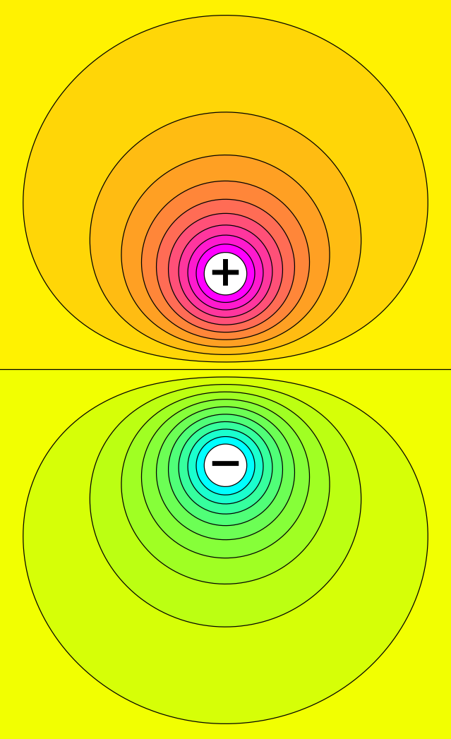
If $f (x, y, z)$ gives the temperature at each point of 3-space, the level surfaces (curves of constant temperature) are called isothermal. In physics, when $f (x, y, z)$ is a potential function, which gives the value of the potential energy at each point of space, the level surfaces are called equipotential or isopotential. Figure 11 shows the electrostatic equipotentials between two electric charges.