In single variable calculus, we learned how to use the chain rule. This rule tells us if and are two differentiable functions then is also a differentiable function and There is an analogous theorem for functions of several variables.
Table of Contents
The Chain Rule for Multivariable Functions
We start with the simplest case for functions of two variables.
Theorem 1. If and are differentiable functions at and if is a differentiable function at , then is differentiable at , and
Show the proof
Hide the proof
Proof: If is given an increment , then , and receive increments , and , and
where . Let’s divide both sides by :
If we let , then because is differentiable and therefore continuous. With the same argument . Because , we conclude .
If is the only independent variable,
Now we just need to plug these expressions in the previous equation:
or
So we have proved the theorem.
Now consider a case where there are other independent variable besides . In this case:
and we have:
Therefore, we have proved the following theorem.
Theorem 2. If and are differentiable functions at and if is a differentiable function at , then is differentiable at , and
Matrix Form of the Chain Rule
We can combine the two equations in the above theorem into a single matrix equation.
This is called the matrix form of the chain rule. Note that the partial derivatives in the first and the last matrices are evaluated at , while the partial derivatives in the second matrix are evaluated at .
When , , and , is dependent variable, and and are independent variables. and are called intermediate variables.
Tree Diagrams
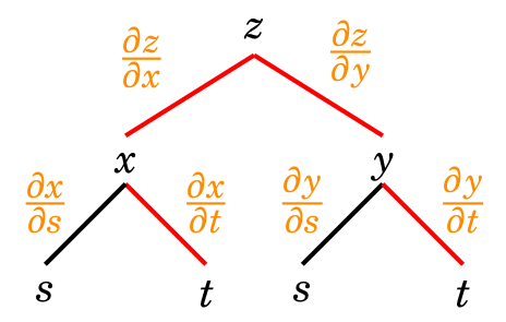
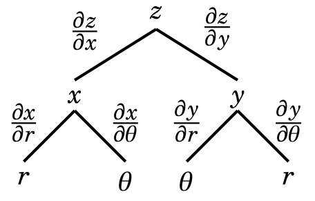
As you will see in the following examples, the chain can take different forms. You can draw a tree diagram to help you determine the correct form of the chain rule for a given problem. Start from the dependent variable, say , and draw branches to the intermediate variables, say and . Then connect the intermediate variables to the independent variables, say and . On each branch write the corresponding partial derivative, for example, . This process is shown in Figure 1. To find , read down each route to , multiply derivatives along the way, and then add the products.
Figure 1. tree diagram
Example 1
If and and find at .
Solution
Method (a) We can plug and into the expression for and then differentiate with respect to :
Now we can easily differentiate with respect to :
For the last step, we can just plug into the above expression:
Method (b): We can use Theorem 1.
When
Therefore:
Sometimes, we cannot use the substitution technique. The following example is one of those situations.
Example 2
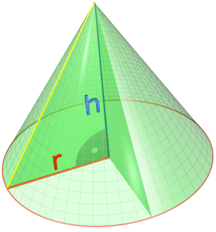
Calculate how fast the volume of a right circular cone is changing if the radius of the base is 5 in and increasing at the rate of 0.1 in/sec, and the altitude of the cone is 12 in and decreasing at rate of 0.5 in/sec.
Solution
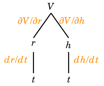
Let be the radius of the base, the altitude, and the volume of the cone. From geometry we know: .
Now and are functions of time, , and we want to find .
We know:
Extension of Theorem 1
Of course, we expand Theorem 1 when is a differentiable function of and are differentiable functions of . Then:
We can write the above equation in a matrix form:
Example 3
Consider two objects moving with time on two paths given by the following equations:
At what rate is the distance between the two objects changing when ?
Solution
The distance between two objects and is:
Here and vary with . For part (a) and (b), we need to find . One method is to plug the formulas of and into the formula of , and make a function of alone. Then you can differentiate it with respect to . We leave this method to you. The second method is to use the chain rule we learned in this section:
Because
we get
and finally
Example 4
If , find the rate of changes of with respect to polar coordinates (find and ).
Solution
In polar coordinates: Method (a): We can write in terms of and and then differentiate with respect to them directly:
Therefore:
Method (b): We can use the chain rule:
Thus:
Example 5
If , and are twice continuously differentiable functions, find .
Solution
According to Theorem 1, we have:
If we differentiate with respect to , we have:
Now and are functions of and , and to find their derivatives with respect to , we apply Theorem 1, with replaced by or . Thus we have: and
Substituting in (*), we have
If , and are twice continuously differentiable functions, find and
Solution
Finding is easy. We just need to replace by in Eq. (**) in the previous example. Therefore:
The process of finding is similar to the process of finding in the previous example. To find , we start from that we know from Theorem 2:
Then we differentiate with respect to :
Again and are two functions of and , therefore:
Substituting the above expressions in (**), we get:
Obviously (***) reduces to (*) if we put .
Example 7
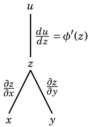
If where is twice continuously differentiable, express in polar coordinates.
Solution
Here we assume , and and we want to find in terms of the first and second partial derivates of with respect to and . Therefore in this example, and are independent variables and and are intermediate variables. To this end, we can use Eq. (*) in the previous example, and replace and with and , and replace and in that equation by and . Therefore: Similarly,
Now we need to find the partial derivates of and with respect to and :
Therefore:
Thus:
As we learned in the previous example, if where is twice continuously differentiable (= has continuous partial derivatives of second order), and if and , then we have :
This is a very important result which has numerous applications in physics, engineering, and solving partial differential equations.
Be Careful About Which Variables Are Held Fixed
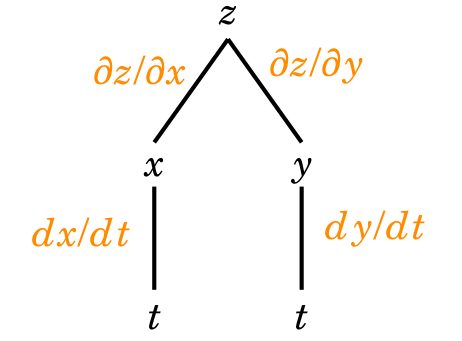
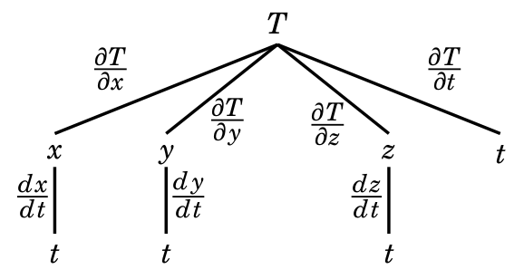
In physics, many quantities such as temperature, density, electrostatic and magnetic fields may vary with time and location. For example, the temperature, , on earth varies with location and time , so we have . If the location where we measure the temperature moves along a path, , and also vary with time. In other words, we have , and . The following tree diagram shows the dependency of temperature on time:
If we wish to find the rate of change of (with time), i.e. , we need to use the chain rule. With the aid of the above diagram, we multiply the corresponding derivatives along each path from to , and add these products together:
Note that is different from . The notation means we have fixed the location and calculate the rate of change of temperature. We may indicate the fact that we have fixed the location and then measured the rate of change of temperate by writing:
Example 8
Suppose in a two dimensional flow, an electrical conductor creates the electrostatic potential field given by: If a particle of the fluid is moving along the path and . Find the rate of change of as seen by the particle when .
Solution
Here we have a function where and also depend on , and we want to find when
When , we have and .
Therefore:
An alternative method is to plug and in the formula of , differentiate with respect to , and then plug in that. However, it is more complicated. Here we skip some calculations and show the results.
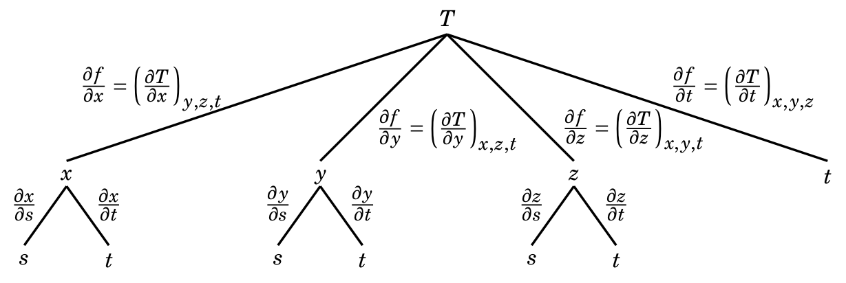
Now consider a case where and , and . In this case, The following tree diagram shows this situation.
If we wish to find , according to the above tree chart, we have:
The above equation might be sometimes written as , but we should note that on the left and on the right have two different meanings. On left we are treating as a constant, and on right we are treating and as constants. To indicate the difference between them, it would be better to use the notation in Equation (ii) or to write it as:
When there is no ambiguity, we may drop some or all of the subscripts.
Example 9
Given and , find .
Solution
Method (a): According to the tree diagram:
Therefore: Method (b): First we plug in the formula for , and then differentiate with respect to :
Homogeneous Functions
A function is called homogeneous of degree if for any and for all in the domain of :
In other words, a function is homogeneous if we multiply its argument by a factor, its values will be multiplied by some power of this factor. Here are some examples of homogeneous functions:
The function is homogeneous of degree 2 because:
The function is homogeneous of degree 8 because :
(Recall )
The function is homogeneous of degree 0 because:
The function is homogeneous of degree 1 because:
The function is homogeneous of degree -1 because:
The function is NOT homogeneous because in general:
(Recall and )
Theorem 3. Euler’s theorem: If is a homogeneous function of degree then:
In general, if is homogeneous of degree then:
Show the proof
Hide the proof
Proof: We prove it for its simplest form. The proof for its general form is similar.
We know: If we differentiate this equation with respect to . If we place and and use the chain rule, we have:
Because this is true for all , it is true when . Plugging in the above equation, gives .
Let’s differentiate (*) again with respect to:
Here we assumed is twice continuously differentiable or of class , hence . Placing , we have:
Example 10
If is homogeneous of degree and , show:
Solution
According to the chain rule:
Therefore [Because is homogeneous of order , according to Theorem 3 .]
Example 11
Given
find .
Solution
We note that if we put , is homogeneous of degree 2, and . Therefore, using the result of the previous example, we have:
Because , therefore . In this interval . That is .
[1] This relationship is valid only when and but for our purpose it is enough.