3.6 Partial Derivatives

To determine how a function of several variables behaves when we change only one variable, we assign finite values to the other variables and allow only this variable to vary. In this case, the function becomes a function of a single variable. For example, consider a function $z=f(x,y)$, and assign to $y$ a (finite) fixed value of $y=y_0$. The result, $z=f(x,y_0)$, is a function of only $x$. The curve formed by the intersection of the surface $z=f(x,y)$ and the plane $y=y_0$ represents the graph of $z=f(x,y_0)$ (see Fig. 1). Now we can differentiate $z=f(x,y_0)$ like a function of a single variable. What we obtain is called the partial derivative of $f(x,y)$ with respect to $x$ at $(x_0,y_0)$:
$$\underset{h\to 0}{lim}\frac{f(x_0+h,y_0)-f(x_0,y_0)}{h}.$$
To emphasize that we first held $y$ fixed at $y_0$ and then we differentiated with respect to $x$ at $x=x_0$, we use a “curved dee” $\partial$ instead of the regular letter $\text{d}$, and denote the above limit by ${\displaystyle \frac{\partial f}{\partial x}}(x_0,y_0)$.

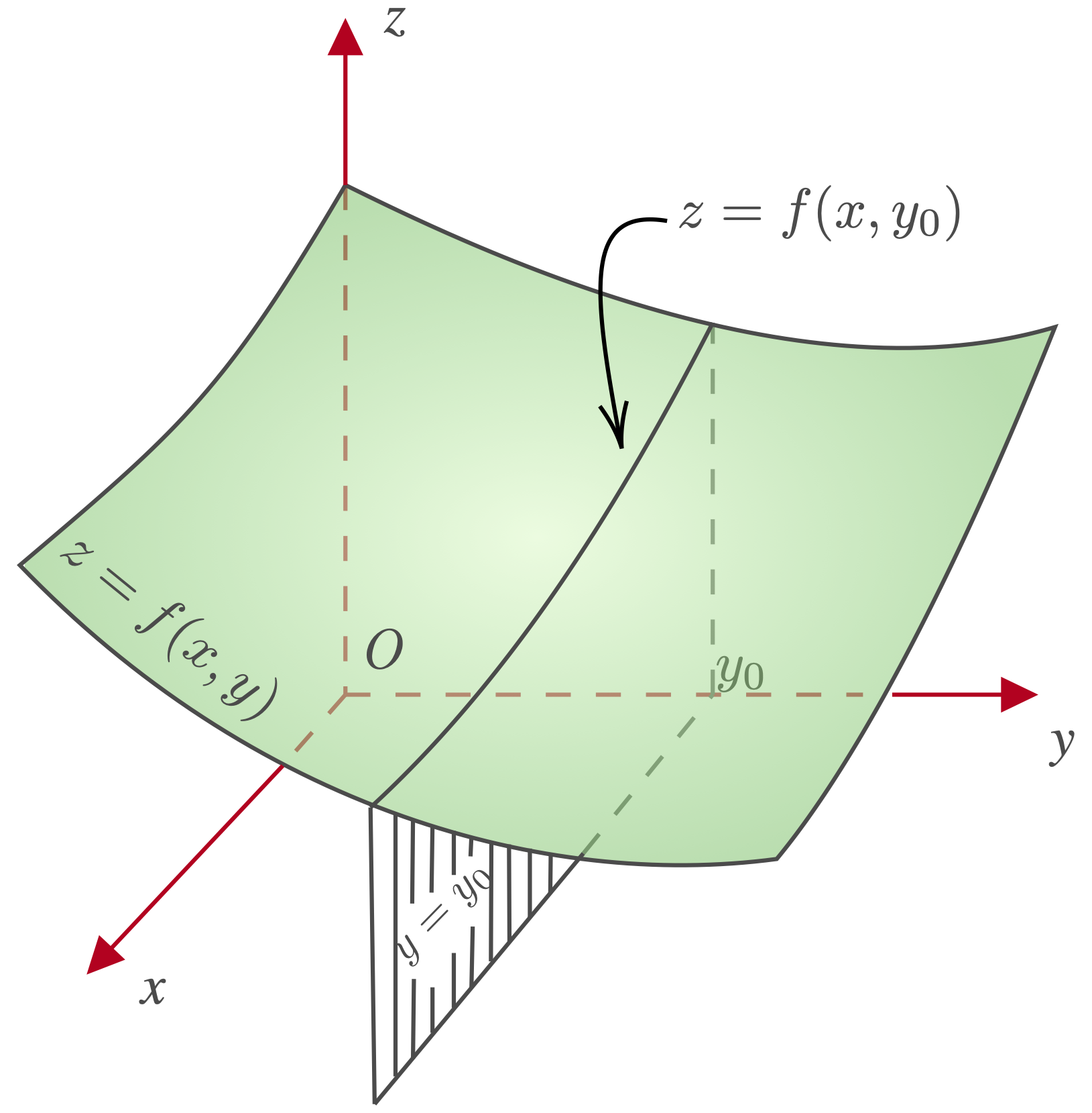Figure 1: section of $z=f(x,y)$.

From single variable calculus, we remember that the derivative is the slope of the tangent line. Here, the partial derivative of $f(x,y)$ with respect to $x$ is the tangent of the angle between the curve $z=f(x,y_0)$ and a line parallel to the $x$-axis at the point $(x_0,y_0,f(x_0,y_0))$. That is, ${\displaystyle \frac{\partial f}{\partial x}}(x_0,y_0)$ is the slope of the surface $z=f(x,y)$ at $(x_0,y_0,f(x_0,y_0))$ in the $x$ direction.

In a similar way, we can hold $x$ constant at $x_0$ and make $f$ a function of $y$ alone, the derivative of which  is the partial derivative of $z=f(x,y)$ with respect to $y$ at $(x_0,y_0)$ and is given by:
$$\frac{\partial f}{\partial y}(x_0,y_0)=\underset{k\to 0}{lim}\frac{f(x_0,y_0+k)-f(x_0,y_0)}{k}.$$

${\displaystyle \frac{\partial f}{\partial x}}(x_0,y_0)$ is slope the slope of the surface $z=f(x,y)$ at $(x_0,y_0,f(x_0,y_0))$ in the $x$ direction. See Fig. 2.

Figure 2: section of  $z=f(x,y)$

If we let $(x_0,y_0)$ vary in the domain of $f(x,y)$ and find the partial derivatives at all points, the partial derivatives become two functions of $x$ and $y$:
$$f_x(x,y)=\frac{\partial f(x,y)}{\partial x},f_y(x,y)=\frac{\partial f(x,y)}{\partial y}$$

• Other common notations of partial derivatives are
  $$\begin{array}{rl}\frac{\partial f(x,y)}{\partial x}=& \frac{\partial }{\partial x}f(x,y)={\left(\frac{\partial f}{\partial x}\right)}_y=f_x(x,y)=f_1(x,y)=D_{x}f(x,y)=D_{1}f(x,y)\\ =& \frac{\partial z}{\partial x}=z_x(x,y)={\partial }_{x}f(x,y)={\partial }_{x}z,\\ \frac{\partial f(x,y)}{\partial y}=& \frac{\partial }{\partial y}f(x,y)={\left(\frac{\partial f}{\partial x}\right)}_x=f_y(x,y)=f_2(x,y)=D_{y}f(x,y)=D_{2}f(x,y)\\ =& \frac{\partial z}{\partial y}=z_y(x,y)={\partial }_{y}f(x,y)={\partial }_{y}z\end{array}$$

• Other common notations, specially in physics and mechanics, are $f_x^{\prime }(x,y)$ or $f_{,x}(x,y)$. Comma or prime is used to emphasize that $x$ is not a subscript.

• If $u=f(x,y,z)$ is a function of $x,y$ and $z$, the first partial derivatives of $f$ with respect to $x,y$, and $z$ are:
  $${\displaystyle \frac{\partial f}{\partial x}}=\underset{h\to 0}{lim}{\displaystyle \frac{f(x+h,y,z)-f(x,y,z)}{h}}$$ $${\displaystyle \frac{\partial f}{\partial y}}=\underset{k\to 0}{lim}{\displaystyle \frac{f(x,y+k,z)-f(x,y,z)}{k}}$$ $${\displaystyle \frac{\partial f}{\partial z}}=\underset{p\to 0}{lim}{\displaystyle \frac{f(x,y,z+p)-f(x,y,z)}{p}}$$

• In general, if $u=f(x_1,x_2,\cdots ,x_n)$ is a function of several variables, we can similarly define its partial derivatives by:

$${\displaystyle \frac{\partial f}{\partial x_k}}={\displaystyle \underset{h\to 0}{lim}{\displaystyle \frac{f(x_1,\cdots ,x_{k-1},x_k+h,x_{k+1},\cdots ,x_n)-f(x_1,\cdots ,x_k,\cdots ,x_n)}{h}}}$$

• To calculate $\partial f/\partial x_k$, we differentiate with respect to $x_k$ in a regular way and deal with the other variables as if they are constants.

• To indicate that a partial derivative of $z=f(x,y)$ has been evaluated at $(x_0,y_0)$, we write:
  $$\frac{\partial f}{\partial x}(x_0,y_0)\text{or}{\frac{\partial f}{\partial x}|}_{(x_0,y_0)}\text{or}{\frac{\partial f}{\partial x}|}_{\genfrac{}{}{0ex}{}{x=x_0}{y=y_0}}\text{or}{f}_x(x_0,y_0)\text{or}{z}_x(x_0,y_0).$$
  In the above notations we can replace $\partial f/\partial x$ with $\partial z/\partial x$.

Examples

Solution

To calculate $\frac{\partial f}{\partial x}(0,0)$ we plug $y=0$, and find a function $g$ of $x$ alone:
$$g(x)=f(x,0)=1-x\Rightarrow \frac{\partial f}{\partial x}(0,0)=g^{\prime }(0)=-1$$

Similarly for $\frac{\partial f}{\partial y}(0,0)$ we plug $x=0$ and find
$$h(y)=f(0,y)=\{\begin{array}{ll}1-y& \text{if }y\ge 0\\ 1-y^2& \text{if }y<0\end{array}$$
where $h(y)$ is a function of single variable. We note that $h$ is continuous at $y=0$ because $\underset{y\to 0^{-}}{lim}h(y)=\underset{y\to 0+}{lim}h(y)=h(0)$. Also
$$h^{\prime }(y)=\{\begin{array}{ll}-1& \text{if }y>0\\ -2y& \text{if }y<0\end{array}.$$
Because $h_{-}‘(0)=[-2y{]}_{y=0}=0$ and $h_{+}^{\prime }(0)=1$ are not equal, $h(y)$ is not differentiable at $y=0$. Therefore, $\frac{\partial f}{\partial y}(0,0)$ does not exist. Graph of $h(y)$ is shown in Fig. 3.

Figure 3