4.6 Infinite Limits

What can we say about functions that grow beyond all bounds?

In this section, we learn:

$lim_{x \to a} f (x) = + \infty$
- The precise definition
$lim_{x \to a} f (x) = - \infty$
- The precise definition
One-sided “infinite” limits
- Logarithmic Functions
Algebraic Operations on Infinite Limits
- Indeterminate Forms $0 \cdot (\pm \infty)$ and $\infty - \infty$
- Indeterminate Form $\pm \infty / (\pm \infty)$

lim_x→a f(x)=+∞

Consider the function $f$ defined by the equation

$f (x) = \frac{1}{(x - 1)^{2}}$

The graph of this function is illustrated in Figure 1.

Figure 1: Graph of

y = \frac{1}{(x - 1)^{2}}

Note that $f$ is not defined at $x = 1$ (division by zero is undefined), but let\textquoteright s consider the values of $f$ when $x$ is close to $1$ . Letting $x$ approach $1$ from both sides, the corresponding values of $f$ are given in the following table.

From this table, we see that as $x$ gets closer and closer to $1$ but never quite equal to $1$ , $f (x)$ becomes indefinitely large; in other words, we can make $f (x)$ as large as we desire if we take $x$ close enough to $1$ .

To express that $f (x)$ increases without bound as $x$ approaches $1$ , we write

$lim_{x \to 1} \frac{1}{(x - 1)^{2}} = + \infty$

Instead of $+ \infty$ , we may simply write $\infty$ .

The equals sign does not mean that the limit exists. Note that $\infty$ is not a number; it is just a symbol for indicating that $f (x)$ indefinitely increases.

Description 1: Let $f$ be a function defined on both sides of $a$ , except possibly at $a$ itself. If we can make $f (x)$ as large as we wish by taking $x$ sufficiently close to $a$ but not equal to $a$ , then we say $f (x)$ approaches $\infty$ as $x$ approaches $a$ (or the limit of $f (x)$ , as $x$ approaches $a$ , is positive infinity and write

$lim_{x \to a} f (x) = + \infty$

Show the Precise Definition of lim_x→a f(x)=+∞

The precise definition is as follows

Definition 1: Let $f$ be a function defined in some deleted neighborhood of $a$ (that is, $f$ is defined for all $x$ on both sides of $a$ except possibly at the number $a$ itself). We say $f (x)$ approaches infinity as $x$ approaches $a$ and write

$lim_{x \to a} f (x) = + \infty$

if for every positive real number $K > 0$ , there exists a $δ > 0$ such that

$f (x) > K whenever 0 < | x - a | < δ .$

This says $lim_{x \to a} f (x) = \infty$ if for any real number $K > 0$ that you give me, I can determine a $δ$ such that for any $x$ closer to $a$ than $δ$ (except when $x = a$ ), $f (x)$ is above the line $y = K$ . A geometric illustration is shown in Figure 2.

Figure 2:

lim_{x \to a} f (x) = \infty

means given any horizontal line

y = K

, we can determine a

δ > 0

such that

f (x)

lies above the line

y = K

for all

x

closer to

a

than

δ

(but with

x \neq a

lim_x→a f(x)=-∞

Now consider the function $g$ defined by the equation

$g (x) = - \frac{1}{(x - 1)^{2}} .$

The graph of $g (x)$ is shown in Figure 3. We notice that $g (x) = - f (x)$ and as $x$ approaches $1$ from either side, $g (x)$ decreases without bound. In this case we write

$lim_{x \to 1} g (x) = - \infty .$

Figure 3: Graph of

y = \frac{- 1}{(x - 1)^{2}}

Description 2: Let $g$ be a function defined on both sides of $a$ , except possibly at $a$ itself. If we can make $g (x)$ as large negative as we wish by taking $x$ sufficiently close to $a$ but not equal to $a$ , then we say $g (x)$ approaches $- \infty$ as $x$ approaches $a$ (or the limit of $g (x)$ is as $x$ approaches $a$ is infinity and write

$lim_{x \to a} g (x) = - \infty .$

Show the Precise Definition of lim_x→a f(x)=-∞

The precise definition is as follows.

Definition 2: Let $g$ be a function defined in some deleted neighborhood of $a$ (that is, $g$ is defined for all $x$ in some open interval containing $a$ except possibly at the number $a$ itself). We say $g (x)$ approaches minus infinity as $x$ approaches $a$ and write

$lim_{x \to a} g (x) = - \infty$

if for every negative real number $C < 0$ , there exists a $δ > 0$ such that

$g (x) < C whenever 0 < | x - a | < δ .$

One-Sided “Infinite” Limits

One-sided limits can be also defined accordingly. For example, consider the function $h (x)$ defined by the equation

$h (x) = \frac{1}{x - 2} .$

Here we can assign all values to $x$ except $2$ as the denominator becomes zero when $x = 2$ . If $x < 2$ , $h (x)$ is negative and if $x > 2$ , $h (x)$ is positive. The graph of this function is represented in Figure 4.

As $x$ approaches $2$ from the left (through the values that are less than $2$ ), $h (x)$ is negative and decreases without bound; while as $x$ approaches $2$ from right (through values that are larger than $2$ ), $h (x)$ increases without bound. In this case, we write

$lim_{x \to 2^{-}} h (x) = - \infty, and lim_{x \to 2^{+}} h (x) = + \infty .$

Figure 4: Graph of

h (x) = \frac{1}{x - 2}

. As we can see here

lim_{x \to 2^{+}} h (x) = + \infty

and

lim_{x \to 2^{-}} h (x) = - \infty

Example 1

Use the precise definition to prove that

$lim_{x \to - 1^{+}} \frac{2}{x + 1} = + \infty .$

Solution

Suppose $K > 0$ is given. We must show that there is a $δ > 0$ such that

$\frac{2}{x + 1} > K whenever - 1 < x < - 1 + δ .$

Because $K > 0$ and $x + 1 > 0$ when $x > - 1$ [Recall that $x \to - 1^{+}$ means $x$ is approaching $- 1$ through values greater than $- 1$ ], we have

$\frac{x + 1}{2} < \frac{1}{K}$

[Recall property 7 in the Section on Inequalities] or

$x + 1 < \frac{2}{K}$

$x < - 1 + \frac{2}{K} .$

So if we have two restrictions on $x$ : (1) $x > - 1$ that guarantees $x + 1 > 0$ and (2) $x < - 1 + 2 / K$ which are equivalent to

$- 1 < x < - 1 + \frac{2}{K},$

then

$\frac{2}{x + 1} > K .$

That is, if we choose $δ \leq 2 / K$ then

$- 1 < x < - 1 + δ ⟹ \frac{2}{x + 1} > K .$

Let's show that this $δ$ works. If $K > 0$ is given, let $δ = 2 / K$ . If $- 1 < x < - 1 + δ$ then

$0 < x + 1 < δ = \frac{2}{K} (Add 1 to each side)$

$\Rightarrow \frac{1}{x + 1} > \frac{K}{2}$

[Recall property 7 in the Section on Inequalities. For example, $5 > 3$ but $\frac{1}{5} < \frac{1}{3}$ ]

$\Rightarrow \frac{2}{x + 1} > K .$

Therefore

$lim_{x \to - 1^{+}} \frac{2}{x + 1} = + \infty .$

The graph of $y = \frac{2}{x + 1}$ is shown below.

Figure 5: Graph of

y = \frac{1}{x + 1}

. As we can see here

lim_{x \to - 1^{+}} y = + \infty

and

lim_{x \to - 1^{-}} y = - \infty

Logarithmic Functions

Let’s look at the graph of $y = \ln x$ (Figure 6); we realize that

$lim_{x \to 0^{+}} \ln x = - \infty$

But because $\ln x$ is not defined for $x < 0$ , we cannot talk about $lim_{x \to 0^{-}} \ln x$ (and hence neither the two-sided limit $lim_{x \to 0} \ln x$ ).

Figure 6: Graph of

y = \ln x

. It is clear from this graph that

lim_{x \to 0^{+}} \ln x = - \infty

In general,

$lim_{x \to 0^{+}} \log_{b} x = {\begin{cases} - \infty & if b > 1 \\ + \infty & if b < 1 \end{cases} .$

See Figure 7.

Figure 7: Graph of

y = \log_{b} x

. If

b > 1

, then

lim_{x \to 0^{+}} \log_{b} x = - \infty

and if

b < 1

lim_{x \to 0^{+}} \log_{b} x = + \infty .

Algebraic operations

Theorem 1: Let $a$ and $L$ be real numbers. If $lim_{x \to a} g (x) = 0$ and $lim_{x \to a} f (x) = L \neq 0$ then

$lim_{x \to a} \frac{f (x)}{g (x)} = {\begin{cases} + \infty & if L > 0 and g (x) > 0 \\ - \infty & if L > 0 and g (x) < 0 \\ - \infty & if L < 0 and g (x) > 0 \\ + \infty & if L < 0 and g (x) < 0 \end{cases}$

The theorem is also valid for the left and right-hand limits; that is, if we replace $x \to a$ by $x \to a^{-}$ or $x \to a^{+}$ .

In the above theorem, we talk about the sign of $g (x)$ for all $x$ close to $a$ (not in its entire domain); it does not matter if the sign of $g$ changes when $x$ is not very close to $a$ .

We may summarize the above theorem and symbolically write

$\frac{L}{0} = + \infty or - \infty (if L \neq 0)$

Depending on the sign of $L$ and the sign of $g (x)$ for $x$ close to $a$ , x. Recall

$\frac{(+)}{(+)} = \frac{(-)}{(-)} = (+) and \frac{(-)}{(+)} = \frac{(+)}{(-)} = (-) .$

Q: We have been always told that division by zero is not defined but here we simply write $L / 0$ is plus or minus infinity. What’s going on?

A: This is just a symbol for memorizing the above theorem. Also, here the denominator is not exactly zero! The denominator gets closer and closer to $0$ as $x$ gets closer and closer to $a$ , but not equal to $a$ . If $g (x) = 0$ for all $x$ close to $a$ , then the function $h (x) = f (x) / g (x)$ will not be defined near $a$ and so we cannot talk about the limit of $f (x) / g (x)$ when $x$ approaches $a$ .

Show the Proof of Theorem 1

We only prove the first case as the proofs of the other cases are similar. To prove that

$lim_{x \to a} \frac{f (x)}{g (x)} = + \infty,$

when $L > 0$ and $g (x) > 0$ for all $x$ close to $a$ , we need to show that for every number $K > 0$ (no matter how large $K$ is), there exists a $δ > 0$ such that for all $x$

\[\text{if \ }0<|x-a|<\delta\text{\ then \ }\frac{f(x)}{g(x)}>K.\]

Because $lim_{x \to a} f (x) = L > 0$ , by taking $ϵ = \frac{L}{2}$ , we can find a $δ_{1} > 0$ such that for all $x$

$if 0 < | x - a | < δ_{1} then | f (x) - L | < \frac{1}{2} L .$

We know that $| f (x) - L | < L / 2$ is equivalent to

$- \frac{L}{2} < f (x) - L < \frac{L}{2}$

$\frac{L}{2} < f (x) < \frac{3 L}{2}$

So there exists a $δ_{1}$ such that for all $x$

$\begin{matrix} (i) & if 0 < | x - a | < δ_{1} then f (x) > \frac{L}{2} \end{matrix}$

On the other hand, because $lim_{x \to a} g (x) = 0$ , for every $ϵ > 0$ , there exists a $δ_{2} > 0$ such that for all $x$

$\begin{matrix} (ii) & if 0 < | x - a | < δ_{2} then g (x) < ϵ \end{matrix}$

[Because $g (x) > 0$ , in the above statement we replaced $| g (x) - 0 |$ by $g (x)$ ]

Alternatively we can say for all $x$

$\begin{matrix} (iii) & if 0 < | x - a | < δ_{2} then \frac{1}{g (x)} > \frac{1}{ϵ} \end{matrix}$

[see property 7 in the Section on Inequalities]

From statements (i) and (iii), we conclude that for every $ϵ > 0$ , there exists a $δ_{1} > 0$ and a $δ_{2} > 0$ such that for all $x$

$if 0 < | x - a | < δ_{1} and 0 < | x - a | < δ_{2} then \frac{f (x)}{g (x)} > \frac{L / 2}{ϵ}$

Hence, if $ϵ = L / (2 K)$ and $δ = min {δ_{1}, δ_{2}}$ , then for all $x$ if $0 < | x - a | < δ$ , then $\frac{f (x)}{g (x)} > \frac{L / 2}{L / (2 K)} = K,$ which is what we were trying to prove.

It follows from the above theorem that

$lim_{x \to 0^{+}} \frac{1}{x^{n}} = + \infty$

$lim_{x \to 0^{-}} \frac{1}{x^{n}} = {\begin{cases} + \infty & if n is even \\ - \infty & if n is odd \end{cases}$

These limits are also clear from the graph of $y = \frac{1}{x^{n}}$ (see the following figures).


(a) $n$ is odd. $lim_{x \to 0^{-}} \frac{1}{x^{n}} = - \infty$ and $lim_{x \to 0^{+}} \frac{1}{x^{n}} = + \infty$ .	(b) $n$ is even. $lim_{x \to 0} \frac{1}{x^{n}} = + \infty$

Figure 8

Because $\tan x = \sin x / \cos x$ ,

$lim_{x \to π / 2} \sin x = 1, lim_{x \to π / 2^{+}} \cos x = 0$

and $\cos x > 0$ when $- π / 2 < x < π / 2$ , we have

$lim_{x \to {\frac{π}{2}}^{-}} \tan x \overset{\frac{1}{0^{+}} = + \infty}{=} + \infty$

and because $\cos x < 0$ when $π / 2 < x < 3 π / 2$ , we have

$lim_{x \to {\frac{π}{2}}^{+}} \tan x \overset{\frac{1}{0^{-}} = - \infty}{=} - \infty .$

These results are also clear from the graph of $y = \tan x$ . As we can see from Figure 9:

$lim_{x \to {\frac{π}{2}}^{-}} \tan x = + \infty, lim_{x \to {\frac{π}{2}}^{+}} \tan x = - \infty$

Figure 9: In general

lim_{x \to a^{-}} \tan x = + \infty

and

lim_{x \to a^{+}} \tan x = - \infty

for

a = \pm \frac{π}{2}, \pm \frac{3 π}{2}, \pm \frac{5 π}{2}, \dots

Similarly, because $\sec x = \frac{1}{\cos x}$ , as $x$ approaches a zero of cosine from one side, the secant goes to plus infinity or minus infinity (See Figure 10).

Figure 10: As

x

approaches where the cosine function is zero (from one side), the secant function goes to

+ \infty

- \infty

. The zeros of cosine occur at

\pm \frac{π}{2}, \pm \frac{3 π}{2}, \pm \frac{5 π}{2}, \dots

Example 2

Find

(a) $lim_{x \to 2^{-}} \frac{x^{2} - 2 x - 1}{x^{2} - 3 x + 2}$

(b) $lim_{x \to 2^{+}} \frac{x^{2} - 2 x - 1}{x^{2} - 3 x + 2}$

Solution

(a) The limit of the numerator is $- 1$

$lim_{x \to 2^{-}} (x^{2} - 2 x - 1) = 2^{2} - 2 \times 2 - 1 = - 1$

and the limit of the denominator is 0

$lim_{x \to 2^{-}} (x^{2} - 3 x + 2) = 2^{2} - 3 \times 2 + 2 = 0.$

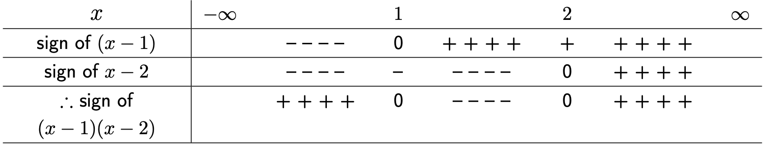
So by Theorem 1, we know the result can be $+ \infty$ or $- \infty$ depending on the sign of numerator (which is negative $- 1 < 0$ ) and the sign of the denominator (which we need to find) as $x \to 2^{-}$ .

To determine the sign of the denominator, we construct a sign table:

$x^{2} - 3 x + 2 = (x - 2) (x - 1)$

so there are two roots $x = 2$ and $x = 1$

From the above table, we see that the denominator is negative as $x$ approaches $2$ from the left. Because the limit of the numerator is $- 1 < 0$ , we obtain

$lim_{x \to 2^{-}} \frac{x^{2} - 2 x - 1}{x^{2} - 3 x + 2} = + \infty .$

“Symbolically” we may write

$\frac{- 1}{0^{-}} = + \infty .$

As in part (a), the limit of the numerator is $- 1 < 0$ and the limit of the denominator is $0$ but from the above sign table we see that the denominator is approaching zero through positive values. Therefore

$lim_{x \to 2^{+}} \frac{x^{2} - 2 x - 1}{x^{2} - 3 x + 2} = - \infty .$

“Symbolically” we may write

$\frac{- 1}{0^{+}} = - \infty .$

The graph of $y = \frac{x^{2} - 2 x - 1}{x^{2} - 3 x + 2}$ is illustrated in the following figure.

Figure 11: Graph of

y = \frac{x^{2} - 2 x - 1}{x^{2} - 3 x + 2}

Example 3

Find

(a) $lim_{x \to 2^{-}} \frac{⌊ x ⌋ - 2}{x - 2}$

(b) $lim_{x \to 2^{+}} \frac{⌊ x ⌋ - 2}{x - 2}$

where $y = ⌊ x ⌋$ is the greatest integer function (also called the floor function). The other notation for $⌊ x ⌋$ is $[[x]]$ .

Solution

(a) When $1 \leq x < 2$ , $⌊ x ⌋ = 1$ . Therefore $lim_{x \to 2^{-}} ⌊ x ⌋ = 1$ and hence $lim_{x \to 2^{-}} (⌊ x ⌋ - 2) = - 1$ . Furthermore, $lim_{x \to 2^{-}} (x - 2) = 2 - 2 = 0$ and $x - 2$ is approaching 0 through negative numbers

$x - 2 < 0 for x < 2.$

Therefore, by Theorem 1, we have

$lim_{x \to 2^{-}} \frac{⌊ x ⌋ - 2}{x - 2} = + \infty .$

“Symbolically” we may write

$\frac{- 1}{0^{-}} = + \infty .$

(b) When $2 \leq x < 3$ , $⌊ x ⌋ = 2$ . Therefore as $x$ is close to 2 but larger than 2, $⌊ x ⌋ - 2$ is exactly zero but $x - 2$ is a small quantity close to zero. If we divide the number zero by any small number (not equal to zero), we get exactly zero. To understand this reasoning better, consider the following table.

$\begin{array}{cccccc} x & \dots & 2.001 & 2.01 & 2.1 & 2.5 \\ ⌊ x ⌋ - 2 & \dots & 0 & 0 & 0 & 0 \\ x - 2 & \dots & 0.001 & 0.01 & 0.1 & 0.5 \\ \frac{⌊ x ⌋ - 2}{x - 2} & \dots & 0 & 0 & 0 & 0 \end{array}$

The graph of $y = \frac{⌊ x ⌋ - 2}{x - 2}$ is shown below.

Figure 12: Graph of

y = \frac{⌊ x ⌋ - 2}{x - 2}

. From this graph we can see that

lim_{x \to 2^{-}} \frac{⌊ x ⌋ - 2}{x - 2} = \infty

and

lim_{x \to 2^{+}} \frac{⌊ x ⌋ - 2}{x - 2} = 0

Example 4

Find
(a) $lim_{x \to 3^{+}} \frac{\sqrt{x^{2} - 9}}{x - 3}$

(b) $lim_{x \to 3^{-}} \frac{\sqrt{9 - x^{2}}}{x - 3}$

Solution

(a) Substituting $x = 3$ into the given expression results in the indeterminate form $0 / 0$ . As $x$ approaches 3 through values greater than 3, $x - 3 > 0$ . Therefore, we can write $x - 3 = \sqrt{(x - 3)^{2}} = \sqrt{x - 3} \sqrt{x - 3}$ [Recall that $\sqrt{t^{2}} = | t |$ . Here $\sqrt{(x - 3)^{2}} = | x - 3 |$ but $x - 3 > 0$ . So $| x - 3 | = x - 3$ ]. Also $\sqrt{x^{2} - 9} = \sqrt{(x - 3) (x + 3)}$ [Recall $A^{2} - B^{2} = (A - B) (A + B)$ ]. Because here $x - 3 > 0$ and $x + 3 > 0$ , we have $\sqrt{(x - 3) (x + 3)} = \sqrt{x - 3} \sqrt{x + 3} .$ Therefore $\begin{aligned} lim_{x \to 3^{+}} \frac{\sqrt{x^{2} - 9}}{x - 3} & = lim_{x \to 3^{+}} \frac{\sqrt{x - 3} \sqrt{x + 3}}{\sqrt{x - 3} \sqrt{x - 3}} \\ = lim_{x \to 3^{+}} \frac{\sqrt{x + 3}}{\sqrt{x - 3}} \end{aligned}$ By direct substitution, the limit of the numerator is $\sqrt{6}$ and the limit of the denominator is 0. The denominator approaches zero through positive numbers [the square root is always positive]. Therefore by Theorem 1, $lim_{x \to 3^{+}} \frac{\sqrt{x + 3}}{\sqrt{x - 3}} \overset{[\frac{\sqrt{6}}{0^{+}}]}{=} + \infty .$ The graph of $y = \sqrt{x^{2} - 9} / (x - 3)$ is shown in Figure 12.

Figure 13: Graph of

y = \frac{\sqrt{x^{2} - 9}}{x - 3}

(b) Similar to part (a), direct subsitution yields the indeterminate form 0/0. As $x \to 3^{-}$ , $x - 3 < 0$ . Thus $\sqrt{(3 - x)^{2}} = | 3 - x | = 3 - x$ or $x - 3 = - \sqrt{3 - x} \sqrt{3 - x} .$ Therefore $\begin{aligned} lim_{x \to 3^{-}} \frac{\sqrt{9 - x^{2}}}{x - 3} & = lim_{x \to 3^{-}} \frac{\sqrt{(3 - x) (3 + x)}}{- \sqrt{3 - x} \sqrt{3 - x}} \\ = lim_{x \to 3^{-}} \frac{\sqrt{3 - x} \sqrt{3 + x}}{- \sqrt{3 - x} \sqrt{3 - x}} \\ = lim_{x \to 3^{-}} \frac{\sqrt{3 + x}}{- \sqrt{3 - x}} . \end{aligned}$ By direct subsitution the limit of the numerator is $\sqrt{6}$ , and the limit of the denomiator is zero. The denominator approaches zero through negative values. Therefore, by Theorem 1 $lim_{x \to 3^{-}} \frac{\sqrt{3 + x}}{- \sqrt{3 - x}} \overset{[\frac{\sqrt{6}}{0^{-}}]}{=} - \infty .$ The graph of $y = \sqrt{9 - x^{2}} / (x - 3)$ is shown in Figure 13.

Figure 14: Graph of

y = \frac{\sqrt{9 - x^{2}}}{x - 3}

Because $+ \infty$ and $- \infty$ are not numbers, the Limit Laws do not apply for infinite limits. If we have infinite limits we can use the following theorem instead.

Theorem 2: (a) If $lim_{x \to a} f (x) = L$ and $lim_{x \to a} g (x) = + \infty$ , then $lim_{x \to a} [f (x) + g (x)] = + \infty$ and $lim_{x \to a} [f (x) g (x)] = {\begin{cases} + \infty & if L > 0 \\ - \infty & if L < 0 \end{cases}$ (b) If $lim_{x \to a} f (x) = L$ and $lim_{x \to a} g (x) = - \infty$ , then $lim_{x \to a} [f (x) + g (x)] = - \infty$ and $lim_{x \to a} [f (x) g (x)] = {\begin{cases} - \infty & if L > 0 \\ + \infty & if L < 0 \end{cases}$ (c) If $lim_{x \to a} f (x) = + \infty$ and $lim_{x \to a} g (x) = + \infty$ , then $lim_{x \to a} [f (x) + g (x)] = + \infty$ and $lim_{x \to a} [f (x) g (x)] = + \infty$ (d) If $lim_{x \to a} f (x) = - \infty$ and $lim_{x \to a} g (x) = - \infty$ , then $lim_{x \to a} [f (x) + g (x)] = - \infty$ and $lim_{x \to a} [f (x) g (x)] = + \infty$

The theorem is valid if we replace $x \to a$ by $x \to a^{+}$ or $x \to a^{-}$ .

We may summarize the above theorem and say

(1) $L + (\pm \infty) = \pm \infty$ (2)

$L (\neq 0) \times (\pm \infty) = {\begin{cases} \pm \infty & if L > 0 \\ \mp \infty & if L < 0 \end{cases}$ (3) $(\pm \infty) \cdot (\pm \infty) = + \infty, (\pm \infty) \cdot (\mp \infty) = - \infty$ (4) $\infty + \infty = + \infty, - \infty - \infty = - \infty .$

For example, because $lim_{x \to 0} - 3 = - 3$ and $lim_{x \to 0} \frac{1}{x^{2}} = + \infty$ , it follows from the above theorem that $lim_{x \to 0} (- 3 + \frac{1}{x^{2}}) = - 3 + \infty = + \infty$ and $lim_{x \to 0} (\frac{- 3}{x^{2}}) = - 3 \cdot (+ \infty) = - \infty .$

Indeterminate Forms 0·∞ and ∞ – ∞

Note that Theorem 2 does not say anything about $0 \cdot (\pm \infty)$ or $\infty - \infty$ : $0 \cdot (\pm \infty) = ? or \infty - \infty = ?$ In fact, we say the cases $0 \cdot (\pm \infty)$ and $\infty - \infty$ are “indeterminate limits.” Let’s look at them this way: We know $\frac{L}{0} = + \infty or - \infty$ So this implies that $0 \cdot (\pm \infty)$ can be any number $L$ , and we need to evaluate each limit case by case. On the other hand because $L + (\pm \infty) = \pm \infty$ we may conclude that $\pm \infty - (\pm \infty)$ can have any value.
Examples showing that an indeterminate limit may take any value
Hide the examples

Note $lim_{x \to 0} x = lim_{x \to 0} x^{2} = lim_{x \to 0} x^{3} = 0$ , and $lim_{x \to 0} \frac{1}{x^{2}} = 0$ , but $lim_{x \to 0} (x \cdot \frac{1}{x^{2}}) = lim_{x \to 0} \frac{1}{x} = {\begin{cases} lim_{x \to 0^{+}} \frac{1}{x} = + \infty & right-hand limit \\ lim_{x \to 0^{-}} \frac{1}{x} = - \infty & left-hand limit \end{cases}$ $lim_{x \to 0} (x^{2} \cdot \frac{1}{x^{2}}) = lim_{x \to 0} 1 = 1$ $lim_{x \to 0} (x^{3} \cdot \frac{1}{x^{2}}) = lim_{x \to 0} x = 0.$ Also $lim_{x \to 0} (4 - \frac{1}{x^{2}}) = 4 - \infty = - \infty$ , and $lim_{x \to 0} \frac{1}{x^{2}} = lim_{x \to 0} \frac{1}{x^{4}} = \infty$ , but $lim_{x \to 0} (\frac{1}{x^{4}} + (4 - \frac{1}{x^{2}})) = lim_{x \to 0} (\frac{1 + 4 x^{2} - x^{2}}{x^{4}}) = [\frac{1}{0^{+}}] = + \infty,$ and $lim_{x \to 0} (\frac{1}{x^{2}} + (4 - \frac{1}{x^{2}})) = lim_{x \to 0} 4 = 4.$
Because limits of the form $0 \cdot (\pm \infty)$ or $\infty - \infty$ may take any value that we cannot predict in advance, we call them indeterminate.

Because $L / 0 = + \infty$ or $- \infty$ , you may think that $L / (\pm \infty) = 0$ . Although $L / 0 = \pm \infty$ is just a symbol and hence does not imply $L / (\pm \infty) = 0$ , the following theorem tells us this conclusion is valid.

Theorem 3: If $lim_{x \to a} f (x) = L$ and $lim_{x \to a} g (x) = + \infty$ or $lim_{x \to a} g (x) = - \infty$ then $lim_{x \to a} \frac{f (x)}{g (x)} = 0.$

Symbolically we may express the above theorem as

$\frac{L}{\pm \infty} = 0.$

Any number divided by a very large (positive or negative) number becomes approximately zero. For example, 2 divided by 1,000,000 is $0.000002 \approx 0$ and 7 divided by $- 100, 000$ is $- 0.00007 \approx 0$ .

Note that $\infty$ is not a number, and $L / \infty = 0$ is just a symbol to memorize the above theorem. Also the following expression helps us remember the two above theorems. $\frac{L}{0} = + \infty or - \infty ⟺ \frac{L}{\pm \infty} = 0.$
On the left expression, $L$ must be nonzero because $0 / 0$ is an indeterminate form (see Section [sec:Ch4-Indeterminate-0/0]) but on the right expression $L$ can be zero. Limits of the form $0 / \infty$ are not indeterminate; roughly speaking $\frac{0}{\infty} = 0 \cdot \frac{1}{\infty} = 0 \cdot 0 = 0.$
On the right, we may replace $L$ with $+ \infty$ or $- \infty$ and the result is still value, because roughly speacking $\frac{(\pm \infty)}{0} = (\pm \infty) \cdot \frac{1}{0}$ $1 / 0$ is $+ \infty$ or $- \infty$ , and infinity multiplied by infinity is infinity. On the other hand, on the right hand side, we cannot replace $L$ with infinity.

Indeterminate Form ∞ / ∞

Theorem 3 does not tell us anything about $\pm \infty / \pm \infty$ . This is another indeterminate form $\frac{\pm \infty}{\pm \infty} = ?$ In fact, we saw $L \cdot (\pm \infty) = + \infty or - \infty$ so $(\pm \infty) / (\pm \infty)$ can be any number $L$ .

We will learn how to deal with limits of the indeterminate forms $0 \cdot (\pm \infty), \infty - \infty$ , and $(\pm \infty) / (\pm \infty)$ in Section 4.10. Finding limits of the indeterminate form $0 / 0$ was discussed in Section 4.5.

Example 5

Find
(a) $lim_{x \to 2^{+}} \frac{\ln (x - 2)}{2 - x}$

(b) $lim_{x \to 2^{-}} \frac{\ln (x - 2)}{2 - x}$

(d) $lim_{x \to 2^{-}} \frac{2 - x}{\ln (x - 2)} .$

Solution

(a) Recall the graph of $y = \ln x$ (Figure [6]). Now if we shift it 2 units to the right, we obtain the graph of $y = \ln (x - 2)$ . As $x$ approaches 2 through values greater than 2 $(x \to 2^{+})$ , $\ln (x - 2)$ is large and negative. That is, $lim_{x \to 2^{+}} \ln (x - 2) = - \infty .$ The function $y = 2 - x$ or $y = - x + 2$ is a polynomial and thus we can simply substitute 2 for $x$ in its expression $lim_{x \to 2^{+}} (2 - x) = 2 - 2 = 0.$ However, when $x$ is greater than $2$ , $2 - x$ approaches 0 through negative values $x > 2 ⟹ 2 - x < 0.$ Therefore $lim_{x \to 2^{+}} \frac{1}{2 - x} \overset{[\frac{1}{0^{-}}]}{=} - \infty$ Finally $lim_{x \to 2^{+}} \frac{\ln (x - 2)}{2 - x} = (lim_{x \to 2^{+}} \ln x) (lim_{x \to 2^{+}} \frac{1}{2 - x}) = (- \infty) \cdot (- \infty) = + \infty .$ The graph of $y = \ln (x - 2) / (2 - x)$ is shown in Figure 15.

Figure 15

(b) Because $\ln (x - 2)$ is not defined for $x < 2$ , $x$ cannot approach 2 through values less than 2 and the left-hand limit does not exist.

(c) In part of (a), we saw $lim_{x \to 2^{+}} f (x) = + \infty$ where $f (x) = \frac{\ln (x - 2)}{2 - x} .$ By Theorem 3, $lim_{x \to 2^{+}} \frac{1}{f (x)} = lim_{x \to 2^{+}} \frac{2 - x}{\ln (x - 2)} = 0.$ The graph of $y = (2 - x) / \ln (x - 2)$ is shown in Figure 16. As we can in this figure, the function approaches 0 as $x \to 2^{+}$ .

You may wonder why the function approaches $+ \infty$ , as $x$ approaches to 3 from the left, and the function approaches $- \infty$ as $x$ approaches to 3 from the right. The reason is that the denominator $\ln (x - 2)$ is zero at $x = 3$ , $lim_{x \to 3^{-}} (2 - x) = - 1$ , and $\ln (x - 2)$ is negative when $x$ is less than 3 (for example if $x = 2.99$ , ${\ln (x - 2) |}_{x = 2.99} = \ln 0.99 < 0)$ Thus by Theorem 1 $lim_{x \to 3^{-}} \frac{2 - x}{\ln (x - 2)} \overset{[\frac{- 1}{0^{-}}]}{=} + \infty .$ A similar argument, shows us that $lim_{x \to 3^{+}} \frac{2 - x}{\ln (x - 2)} \overset{[\frac{- 1}{0^{+}}]}{=} - \infty .$

(d) Again because $\ln (x - 2)$ is not defined for $x < 2$ , the left-hand limit does not exist.

lim_x→a f(x)=+∞

Show the Precise Definition of lim_x→a f(x)=+∞

Hide the Precise Definition

lim_x→a f(x)=-∞

Show the Precise Definition of lim_x→a f(x)=-∞

Hide the Precise Definition

One-Sided “Infinite” Limits

Logarithmic Functions

Algebraic operations

Show the Proof of Theorem 1

Hide the Proof

Examples showing that an indeterminate limit may take any value

Hide the examples

limx→a f(x)=+∞

Show the Precise Definition of limx→a f(x)=+∞

Hide the Precise Definition

limx→a f(x)=-∞

Show the Precise Definition of limx→a f(x)=-∞

Hide the Precise Definition

One-Sided “Infinite” Limits

Logarithmic Functions

Algebraic operations

Show the Proof of Theorem 1

Hide the Proof

Examples showing that an indeterminate limit may take any value

Hide the examples

lim_x→a f(x)=+∞

Show the Precise Definition of lim_x→a f(x)=+∞

lim_x→a f(x)=-∞

Show the Precise Definition of lim_x→a f(x)=-∞